Improving search result relevancy on Wikipedia with BM25 ranking
Revised on 17 November 2016
Erik Bernhardson (Engineering)
David Causse (Engineering & Report)
Trey Jones (Engineering & Review)
Mikhail Popov (Analysis & Report)
Deb Tankersley (Product Management)
Chelsy Xie (Review)
Originally published on 11 October 2016
{ RMarkdown Source | Analysis Codebase }
Revision Notes: In the original version of this report, some of the engagement and PaulScore calculations did not filter out searches with zero results. In this revised version, we added a filter that only keeps searches with some results (since that means users actually have something to click on). The clickthrough rates and PaulScores are slightly higher all around, so the overall conclusions are the same, but we still wanted this report to be as accurate as it can be.
Executive Summary
In order to improve the relevancy of search results, Discovery’s Search team has decided to test a new document ranking function called BM25, which would replace the Lucene classic similarity that is currently used. We saw the following results from our analysis:
- █ Same “all field” query builder as control group but using BM25 as similarity function
- For searches made by users in this group, we use the same query builder as we use for the control group, but we switched the similarity function to BM25 and employ a weighted sum for the incoming links query independent factor (QIF). Users in this group were less likely to click on the 1st search result and instead more likely to click on the second search result. They were also more likely to reformulate their query. With regards to zero results rate (ZRR), PaulScore, and engagement, users in this group were very similar to users in the control group.
- █ Using per-field query building with incoming links as QIF
- For searches made by users in this group, we use BM25 similarity and switch to a per-field query builder using only incoming links as a query independent factor. This group had the second-highest PaulScores and engagement in searches where the user reformulated their query. Users in this group were more likely to click on the first search result than users in the control group.
- █ Using per-field query builder with incoming links and pageviews as QIFs
- Similar to the group described above but we added pageviews as an additional query independent factor for searches made by users in this group. This group had the highest PaulScores and engagement, both in searches where the user reformulated their query and in searches without query reformulation. Users in this group were a lot more likely to click on the first search result than users in the control group.
- █ Track typos in first 2 characters
- Similar to the group described above, but with an additional field to track typos in the first two characters. This group had the lowest ZRR, and its ZRR was significantly smaller than the control group’s ZRR. This group also had the smallest proportion of searches where the user reformulated their query. Users in this group were a lot more likely to click on the first search result than users in the control group, but had lowest overall engagement with the search results.
We recommend switching to BM25 ranking with incoming links (and possibly pageviews) as query-independent factors, as this configuration appears to give users results that are more relevant and that they engage with more (especially the first search result).
Background
The Discovery department’s mission is to help users discover and access knowledge on Wikipedia and other Wikimedia projects. One of the goals of Discovery’s Search team is to improve the relevance of results when users search Wikipedia and its sister projects. Currently, our search engine uses Lucene classic similarity to rank articles using term frequency–inverse document frequency (tf–idf). To improve the search results, we decided to try a new document-ranking function: Okapi BM25 (BM stands for Best Matching). To assess the efficacy of the proposed switch, we ran an A/B test for 10 days and anonymously tracked randomly sampled search sessions. Some users received search results acquired through the Lucene similarity, while others received search results acquired through BM25 with various configurations. We are primarily interested in:
- Zero results rate, the proportion of searches that yielded zero results (smaller is better)
- Users’ engagement with the search results, measured as the clickthrough rate (bigger is better)
- PaulScore, a metric of search results’ relevancy that relies on the position of the clicked result[s] (bigger is better); see PaulScore Definition below for more details
- Query reformulation – one way to think about the strength of our search engine is how many times the user reformulates their query; if a user in the test group has to reformulate their query many more times to get the results they are interested in, then maybe the change is for the worse
Methods
Data
Users who searched English Wikipedia (“enwiki”) had a 1 in 66 chance of being selected for search satisfaction tracking according to our TestSearchSatisfaction2 #15700292 schema. See change 307536 on Gerrit for more details. Those users who were on enwiki and were randomly selected to have their sessions anonymously tracked then had a 2 in 3 chance of being selected for the BM25 test.
Users who were randomly selected for the A/B test were then randomly assigned to one of five groups. For all the groups listed below, we include the normalized discounted cumulative gain (nDCG) score – a measure of ranking quality – computed from ranking data collected through Discernatron, a tool that allows participants to judge the relevance of search results to help the Search team be able to test changes before making them available on-wiki.
- Control Group (tf–idf)
- Identical to what we serve to our users today plus an artificial latency to compensate the fact that we run the other buckets on another data center. (nDCG5 score on Discernatron: 0.2772)
- Same “all field” query builder as control group but using BM25 as similarity function
- For searches made by users in this group, we use the same query builder as we use for the control group but we switched the similarity function to BM25 and employ a weighted sum for the incoming links query independent factor (QIF). We expected this bucket to behave poorly in term of clickthrough compared to the control group. We included this group confirm our assumptions that the current query builder and the “all field” approach is not designed for the BM25 similarity. (nDCG5 score on Discernatron: 0.2689)
- Using per-field query building with incoming links as QIF
- For searches made by users in this group, we use BM25 similarity and switch to a per-field query builder using only incoming links as a query independent factor. This is the best contender according to Discernatron. We expect an increase in clickthrough because it tends rank obvious matches in the top 3. (nDCG5 score on Discernatron: 0.3362)
- Using per-field query builder with incoming links and pageviews as QIFs
- Similar to the group described above but we added pageviews as an additional query independent factor for searches made by users in this group. The weight for pageviews is still very low compared to incoming links and this test is mostly to see how pageviews could affect the ranking. We expect a very minimal difference in behavior compared to group using per-field query building with incoming links as QIF. (nDCG5 score on Discernatron: 0.3359)
- Track typos in first 2 characters
- Similar to the group described above, but with an additional field to track typos in the first two characters. We expect a slight decrease in zero result rate and hope for an increase in clickthrough rate. This test is added to measure the benefit of such a field. The question of interest we hope to answer is: Will this increase in noise provide more annoying suggestions or will it help our users? (This feature can’t be really tested with Discernatron today.)
The “all field” field approach combines raw term frequency and field weights at index time, it creates an artificial field where the content of each field is copied n times:
- A word in the title is copied 20 times
- A word in the title is copied 15 times
At query time, we use this single all weighted field. The per field builder approach combines scores of individual fields at query time.
The full-text (as opposed to auto-complete) searching event logging data was extracted from the database using the following SQL query:
SELECT
  LEFT(`timestamp`, 8) AS date,
  event_subTest AS test_group,
  `timestamp` AS ts,
  event_uniqueId AS event_id,
  event_mwSessionId AS session_id,
  event_searchSessionId AS search_id,
  event_pageViewId AS page_id,
  event_searchToken AS cirrus_id,
  CAST(event_query AS CHAR CHARACTER SET utf8) AS query,
  event_hitsReturned AS n_results_returned,
  event_msToDisplayResults AS load_time,
  CASE WHEN event_action = 'searchResultPage' THEN 'SERP' ELSE 'click' END AS action,
  event_position AS position_clicked
FROM TestSearchSatisfaction2_15700292
WHERE
  LEFT(`timestamp`, 8) >= '20160830' AND LEFT(`timestamp`, 8) <= '20160910'
  AND event_source = 'fulltext'
  AND LEFT(event_subTest, 4) = 'bm25'
  AND (
    (event_action = 'searchResultPage' AND event_hitsReturned IS NOT NULL AND event_msToDisplayResults IS NOT NULL)
    OR
    (event_action = 'click' AND event_position IS NOT NULL AND event_position > -1)
  )
ORDER BY date, wiki, session_id, search_id, page_id, action DESC, timestamp;
Snippet 1: Query used to extract BM25 test data from our event logging database.
Software
We used the statistical analysis software and programming language R[2] to perform this analysis. R packages used the most in this report include ggplot2,[4] dplyr,[5] and binom.[8]
# Install packages used in the report:
install.packages(c("devtools", "tidyverse", "binom"))
devtools::install_github("hadley/ggplot2")
# ^ development version of ggplot2 includes subtitles
devtools::install_github("wikimedia/wikimedia-discovery-polloi")
# ^ for converting 100000 into 100K via polloi::compress()
# Load packages that we will be using in this report:
library(tidyverse) # for ggplot2, dplyr, tidyr, broom, etc.
library(binom) # for Bayesian confidence intervals of proportionsSearch Clustering
When a user searches Wikipedia using query \(Q\) and does not get the results that they were looking for then they might give up, or they might reformulate their query and search for \(Q', Q'', Q'''\), etc., each time fixing a typo, editing a word, or adding new information. For example, if the user searches for the restaurant chain “Buffalo Wild Wings” using the search query “buffalo”, they won’t see the result on the first search results page. The user might go to the second page of results, in which case they would see the result they want, or they might reformulate their query to instead say “buffalo wings”.
First, we computed the Levenshtein (edit) distance (normalized via dividing by the maximum of the two search queries’ lengths). Then we adjusted those normalized distances by the amount that their search results overlapped. Specifically, if \(d_{Q, Q'}\) is the edit distance between queries \(Q\) and \(Q'\) and \(\rho_{Q, Q'} \in [0, 1]\) is the number of results in common normalized via dividing by the minimum of the two result sets’ sizes, then the new distance is: \[{d'}_{Q, Q'} = \frac{d_{Q, Q'}}{10^{\rho_{Q, Q'}}}.\] So if \(Q\) and \(Q'\) are moderately similar but have all results in common, then the new distance is 1/10th of their initially calculated distance, and brings them a lot closer to each other. Another example is if two searches have 1 result out of 20 in common, then \(d' = 10^{-0.05} d = 0.89 d\). If they do not have any results in common, their edit distance is unaffected. After we have calculated the distances between queries in a search session, we use hierarchical agglomerative clustering to group those queries based on their adjusted closeness (similarity). In this report we present an analysis result when employing each of the three linkages (complete, single, and average), since the choice of linkage affects the clustering (see Table 1 for an example).
For example:
| Search query | Single-linkage | Complete-linkage |
|---|---|---|
| brtisth gas | Cluster A | Cluster A |
| brtisth gaz | Cluster A | Cluster A |
| brtisth gazcomapny | Cluster B | Cluster A |
| fusion shell bg group | Cluster C | Cluster B |
Table 1: Example of how choice of linkage affects clustering of queries from a real search session.
overlapping_results <- function(x) {
  if (all(is.na(x))) {
    return(diag(length(x)))
  }
  input <- strsplit(stringr::str_replace_all(x, "[\\[\\]]", ""), ",")
  output <- vapply(input, function(y) {
    temp <- vapply(input, function(z) { length(intersect(z, y)) }, 0L)
    # Normalize by diving by number of possible matches
    # e.g. if two queries have two results each that are
    #      exactly the same, that's worth more than if
    #      two queries have 20 results each but have
    #      only three in common
    temp <- temp/pmin(rep(length(y), length(input)), vapply(input, length, 0L))
    temp[is.na(x)] <- 0L
    return(temp)
  }, rep(0.0, length(input)))
  diag(output) <- 1L
  return(output)
}

cluster_queries <- function(queries, results, linkage = c("complete", "single", "average"), threshold = NULL, debug = FALSE) {
  if (length(queries) < 2) {
    return(1)
  }
  input <- data.frame(query = queries, stringsAsFactors = FALSE)
  x <- do.call(rbind, lapply(input$query, function(x) {
    # Compute for each x in input$query the normalized edit distance from x to input$query:
    normalized_distances <- adist(tolower(x), tolower(input$query), fixed = TRUE)/pmax(nchar(x), nchar(input$query))
    # Return:
    return(normalized_distances)
  }))
  # Decrease distance of queries that share results:
  overlaps <- overlapping_results(results)
  x <- x * (10^(-overlaps))
  # ^ if two queries have the exact same results, we make the new
  #   edit distance 0.1 of what their original edit distance is
  # Create distance object:
  y <- x[lower.tri(x, diag = FALSE)]
  d <- structure(
    y, Size = length(queries), Labels = queries, Diag = FALSE, Upper = FALSE,
    method = "levenshtein", class = "dist", call = match.call()
  )
  clustering_tree <- hclust(d, method = linkage[1])
  # When using average linkage, we may end up with funky trees
  #   that cannot be properly cut. So this logic helps against
  #   errors and yieds NAs instead.
  clusters <- tryCatch(
    cutree(clustering_tree, h = threshold),
    error = function(e) { return(NA) })
  if (all(is.na(clusters))) {
    clusters <- rep(clusters, nrow(input))
    names(clusters) <- input$query
  }
  output <- left_join(
    input,
    data.frame(query = names(clusters),
               cluster = as.numeric(clusters),
               stringsAsFactors = FALSE),
    by = "query")
  if (debug) {
    return(
      list(
        original_distances = x / (10^(-overlaps)),
        overlaps = overlaps,
        modified_distances = d,
        output = output,
        hc = clustering_tree
      )
    )
  }
  return(output$cluster)
}
PaulScore Definition
PaulScore[1] is a measure of search results’ relevancy which takes into account the position of the clicked results, and is computed via the following steps:
- Pick scoring factor \(0 < F < 1\) (larger values of \(F\) increase the weight of clicks on lower-ranked results).
- For \(i\)-th search session \(S_i\) \((i = 1, \ldots, n)\) containing \(m\) queries \(Q_1, \ldots, Q_m\) and search result sets \(\mathbf{R}_1, \ldots, \mathbf{R}_m\):
- For each \(j\)-th search query \(Q_j\) with result set \(\mathbf{R}_j\), let \(\nu_j\) be the query score: \[\nu_j = \sum_{k~\in~\{\text{0-based positions of clicked results in}~\mathbf{R}_j\}} F^k.\]
- Let user’s average query score \(\bar{\nu}_{(i)}\) be \[\bar{\nu}_{(i)} = \frac{1}{m} \sum_{j = 1}^m \nu_j.\]
- Then the PaulScore is the average of all users’ average query scores: \[\text{PaulScore}(F)~=~\frac{1}{n} \sum_{i = 1}^n \bar{\nu}_{(i)}.\]
We can calculate the confidence interval of PaulScore\((F)\) by approximating its distribution via boostrapping.
# PaulScore Calculation
query_score <- function(positions, F) {
   if (length(positions) == 1 || all(is.na(positions))) {
    # no clicks were made
    return(0)
   } else {
     positions <- positions[!is.na(positions)] # when operating on 'events' dataset, SERP events won't have positions
  return(sum(F^positions))
   }
}
# Bootstrapping
bootstrap_mean <- function(x, m, seed = NULL) {
  if (!is.null(seed)) {
    set.seed(seed)
  }
  n <- length(x)
  return(replicate(m, mean(x[sample.int(n, n, replace = TRUE)])))
}
Results
# Import events fetched from MySQL
load(path("data/ab-test_bm25.RData"))
events$test_group <- factor(
  events$test_group,
  levels = c("bm25:control", "bm25:allfield", "bm25:inclinks", "bm25:inclinks_pv", "bm25:inclinks_pv_rev"),
  labels = c("Control Group (tf–idf)", "Same query builder as control group but using BM25 as similarity function", "Using per-field query building with incoming links as QIF", "Using per-field query builder with incoming links and pageviews as QIFs", "Track typos in first 2 characters"))
cirrus <- readr::read_tsv(path("data/ab-test_bm25_cirrus-results.tsv.gz"), col_types = "ccc")
events <- left_join(events, cirrus, by = c("event_id", "page_id"))
rm(cirrus)
The test was deployed on September 1st and ran for 10 days, collecting a total of 119.6K events from 36.2K unique sessions. See Table 2 for counts broken down by test group.
events_summary <- events %>%
  group_by(`Test group` = test_group) %>%
  summarize(`Search sessions` = length(unique(search_id)), `Events recorded` = n()) %>%
  {
    rbind(., tibble(
      `Test group` = "Total",
      `Search sessions` = sum(.$`Search sessions`),
      `Events recorded` = sum(.$`Events recorded`)
    ))
  } %>%
  mutate(`Search sessions` = prettyNum(`Search sessions`, big.mark = ","),
         `Events recorded` = prettyNum(`Events recorded`, big.mark = ","))
events_summary$`Test group` <- paste0("<span class='test-group-", 1:nrow(events_summary), "'>", events_summary$`Test group`, "</span>")
knitr::kable(events_summary, format = "markdown", align = c("l", "r", "r"))| Test group | Search sessions | Events recorded |
|---|---|---|
| Control Group (tf–idf) | 7,297 | 23,484 |
| Same query builder as control group but using BM25 as similarity function | 7,133 | 22,908 |
| Using per-field query building with incoming links as QIF | 7,330 | 24,799 |
| Using per-field query builder with incoming links and pageviews as QIFs | 7,235 | 23,557 |
| Track typos in first 2 characters | 7,161 | 24,868 |
| Total | 36,156 | 119,616 |
Table 2: Counts of sessions anonymously tracked and events collected during the ten-day-long A/B test.
SERP De-duplication
An issue we noticed with the event logging is that when the user goes to the next page of search results or clicks the Back button after visiting a search result, a new page ID is generated for the search results page. The page ID is how we connect click events to search result page events. There is currently a Phabricator ticket (T146337) for addressing these issues. For this analysis, we de-duplicated by connecting search engine results page (SERP) events that have the exact same search query, and then connected click events together based on the SERP connectivity.
# Correct for when user uses pagination or uses back button to go back to SERP after visiting a result.
# Start by assigning the same page_id to different SERPs that have exactly the same query:
temp <- events %>%
  filter(action == "SERP") %>%
  group_by(session_id, search_id, query) %>%
  mutate(new_page_id = min(page_id)) %>%
  ungroup %>%
  select(c(page_id, new_page_id)) %>%
  distinct
# We also need to do the same for associated click events:
events <- left_join(events, temp, by = "page_id"); rm(temp)
# Find out which SERPs are duplicated:
temp <- events %>%
  filter(action == "SERP") %>%
  arrange(new_page_id, ts) %>%
  mutate(dupe = duplicated(new_page_id, fromLast = FALSE)) %>%
  select(c(event_id, dupe))
events <- left_join(events, temp, by = "event_id"); rm(temp)
events$dupe[events$action == "click"] <- FALSE
# Remove duplicate SERPs and re-sort:
events <- events[!events$dupe & !is.na(events$new_page_id), ] %>%
  select(-c(page_id, dupe)) %>%
  rename(page_id = new_page_id) %>%
  arrange(date, session_id, search_id, page_id, desc(action), ts)
# Summarize on a page-by-page basis:
searches <- events %>%
group_by(`test group` = test_group, session_id, search_id, page_id) %>%
filter("SERP" %in% action) %>% # filter out searches where we have clicks but not SERP events
summarize(ts = ts[1], query = query[1],
results = ifelse(n_results_returned[1] > 0, "some", "zero"),
clickthrough = "click" %in% action,
`first clicked result's position` = ifelse(clickthrough, position_clicked[2], NA),
`result page IDs` = result_pids[1],
`Query score (F=0.1)` = query_score(position_clicked, 0.1),
`Query score (F=0.5)` = query_score(position_clicked, 0.5),
`Query score (F=0.9)` = query_score(position_clicked, 0.9)) %>%
arrange(ts)
# Cluster queries
safe_clust <- function(search_id, page_ids, queries, results, threshold, linkage) {
clusters <- cluster_queries(queries, results, linkage, threshold)
if (length(clusters) != length(page_ids)) {
stop("Number of cluster labels does not match number of searches for search session ", unlist(search_id)[1])
} else {
return(clusters)
}
}After de-duplicating, we collapsed 101.1K (SERP and click) events into 70K searches.
searches <- searches %>%
  group_by(`test group`, session_id, search_id) %>%
  mutate(
    cluster_single = safe_clust(search_id, page_id, query, `result page IDs`, 0.301, "single"),
    cluster_average = safe_clust(search_id, page_id, query, `result page IDs`, 0.433, "average"),
    cluster_complete = safe_clust(search_id, page_id, query, `result page IDs`, 0.45, "complete")
  )
most_common <- function(x) {
if (all(is.na(x))) {
return(as.character(NA))
} else {
return(names(sort(table(x), decreasing = TRUE))[1])
}
}
summarize_reformulations <- function(grouped_data) {
return({
grouped_data %>%
# Count number of similar searches made in a single search session
# (multiple search sessions per MW session allowed)
summarize(
reformulations = n() - 1,
clickthrough = any(clickthrough),
results = ifelse("some" %in% results, "some", "zero"),
`most popular position clicked first` = most_common(`first clicked result's position`),
`Cluster score (F=0.1)` = mean(`Query score (F=0.1)`, na.rm = TRUE),
`Cluster score (F=0.5)` = mean(`Query score (F=0.5)`, na.rm = TRUE),
`Cluster score (F=0.9)` = mean(`Query score (F=0.9)`, na.rm = TRUE)
) %>%
ungroup
})
}
set.seed(0) # for reproducibility
query_reformulations_single <- searches %>%
group_by(`test group`, session_id, search_id, cluster = cluster_single) %>%
summarize_reformulations
query_reformulations_complete <- searches %>%
group_by(`test group`, session_id, search_id, cluster = cluster_complete) %>%
summarize_reformulations
query_reformulations_average <- searches %>%
ungroup %>%
filter(!is.na(cluster_average)) %>%
group_by(`test group`, session_id, search_id, cluster = cluster_average) %>%
summarize_reformulations
query_reformulations <- bind_rows(
"Queries grouped via average linkage" = query_reformulations_average,
"Queries grouped via complete linkage" = query_reformulations_complete,
"Queries grouped via single linkage" = query_reformulations_single,
.id = "linkage")
rm(query_reformulations_average, query_reformulations_complete, query_reformulations_single)Query Reformulation
As mentioned in the Methods section, we used hierarchical clustering to group similar searches together. That is, if the edit distance between two search queries is small enough and the search result sets overlap, those searches are probably the user reformulating their query. In Figures 1 and 2, we see proportions of searches that were reformulations, according to three different ways to group searches. The second group (“same query builder as control group but using BM25”) had the highest proportion of searches where the user reformulated their query at least once, and this difference is statistically significant. According to clustering via single linkage, the last group (BM25 with incoming links and tracking typos) had the lowest proportion of query reformulations.
# Calculate proportions of searches with 0, 1, 2, 3+ query reformulations
query_reformulations %>%
  mutate(`query reformulations` = forcats::fct_lump(factor(reformulations), 3, other_level = "3+")) %>%
  group_by(linkage, `test group`, `query reformulations`) %>%
  tally %>%
  mutate(proportion = n/sum(n)) %>%
  ggplot(aes(x = `query reformulations`, y = proportion, fill = `test group`)) +
  geom_bar(stat = "identity", position = "dodge") +
  scale_y_continuous(labels = scales::percent_format()) +
  scale_fill_brewer("Test Group", palette = "Set1", guide = guide_legend(ncol = 2)) +
  facet_wrap(~ linkage, ncol = 3) +
  labs(y = "Proportion of searches", x = "Approximate number of query reformulations per search session",
       title = "Number of query reformulations by test group and linkage",
       subtitle = "Queries were grouped via hierarchical clustering using average/complete/single linkage and edit distance adjusted by search results in common") +
  theme_minimal(base_family = "Lato") +
  theme(legend.position = "bottom",
        strip.background = element_rect(fill = "gray90"),
        panel.border = element_rect(color = "gray30", fill = NA))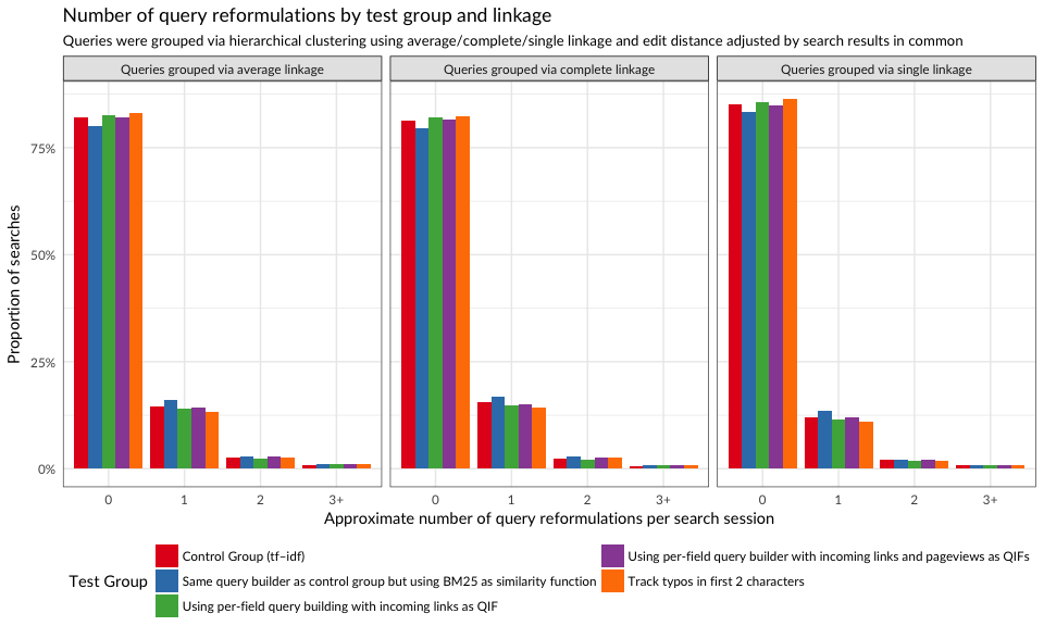
Figure 1: Proportions of searches with 0, 1, 2, and 3+ query reformulations.
# Calculate proportion of searches where user reformulated their query
reformulation_counts <- query_reformulations %>%
  group_by(linkage, `test group`) %>%
  summarize(`searches with query reformulations` = sum(reformulations > 0),
            searches = n(),
            proportion = `searches with query reformulations`/searches) %>%
  ungroup
reformulation_counts <- cbind(
  reformulation_counts,
  as.data.frame(
    binom:::binom.bayes(
      reformulation_counts$`searches with query reformulations`,
      n = reformulation_counts$searches)[, c("mean", "lower", "upper")]
  )
)
reformulation_counts %>%
ggplot(aes(x = 1, y = mean, color = `test group`)) +
geom_hline(aes(yintercept = mean), linetype = "dashed", color = RColorBrewer::brewer.pal(3, "Set1")[1],
data = filter(reformulation_counts, `test group` == "Control Group (tf–idf)")) +
geom_pointrange(aes(ymin = lower, ymax = upper), position = position_dodge(width = 1)) +
scale_y_continuous(labels = scales::percent_format(),
breaks = seq(.10, .24, 0.01),
minor_breaks = seq(.10, .24, 0.005),
expand = c(0.01, 0.01)) +
scale_color_brewer("Test Group", palette = "Set1", guide = guide_legend(ncol = 2)) +
facet_wrap(~ linkage, ncol = 3) +
geom_text(aes(label = sprintf("%.1f%%", 100 * proportion), y = upper + 0.0025, vjust = "bottom"),
position = position_dodge(width = 1)) +
labs(y = "% of searches with query reformulations", x = NULL,
title = "Searches with reformulated queries by test group (and linkage)",
subtitle = "Queries were grouped via hierarchical clustering using average/complete/single linkage and edit distance adjusted by search results in common") +
theme_minimal(base_family = "Lato") +
theme(legend.position = "bottom",
panel.grid.major.x = element_blank(),
panel.grid.minor.x = element_blank(),
axis.ticks.x = element_blank(),
axis.text.x = element_blank(),
strip.background = element_rect(fill = "gray90"),
panel.border = element_rect(color = "gray30", fill = NA))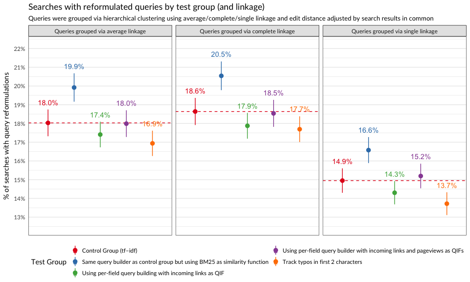
Figure 2: Proportions of searches where user reformulated their query.
Zero Results Rate
In Figure 3, we see that zero results rate (ZRR) was not so different between the groups. The test group where we tracked typos in first two characters had a significantly lower ZRR, but perhaps at the cost of relevance and engagement with the results (see Figure 5).
zrr_pages <- searches %>%
  group_by(`test group`, results) %>%
  tally %>%
  spread(results, n) %>%
  mutate(`zero results rate` = zero/(some + zero)) %>%
  ungroup
zrr_pages <- cbind(zrr_pages, as.data.frame(binom:::binom.bayes(zrr_pages$zero, n = zrr_pages$some + zrr_pages$zero)[, c("mean", "lower", "upper")]))
zrr_pages %>%
ggplot(aes(x = `test group`, y = `mean`, color = `test group`)) +
geom_hline(
yintercept = zrr_pages$`mean`[zrr_pages$`test group` == "Control Group (tf–idf)"],
linetype = "dashed", color = "gray50") +
geom_pointrange(aes(ymin = lower, ymax = upper)) +
scale_x_discrete(limits = rev(levels(events$test_group))) +
scale_y_continuous(labels = scales::percent_format()) +
scale_color_brewer("Test Group", palette = "Set1", guide = FALSE) +
labs(x = NULL, y = "Zero Results Rate",
title = "Proportion of searches that did not yield any results, by test group",
subtitle = "With 95% credible intervals. Dashed line represents the baseline (ZRR of the control group).") +
geom_text(aes(label = sprintf("%.2f%%", 100 * `zero results rate`),
vjust = "bottom", hjust = "center"), nudge_x = 0.1) +
coord_flip() +
theme_minimal(base_family = "Lato")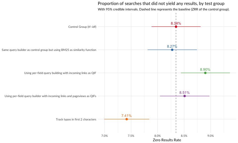
Figure 3: Zero results rate is the proportion of searches in which the user received zero results.
PaulScore
In Figure 4, we see that the test groups that used BM25 with incoming links and pageviews as query-independent factors had higher PaulScores, which indicates that the results were more relevant.
set.seed(0) # for reproducibility
paulscores <- searches %>%
  ungroup %>%
  filter(results == "some") %>%
  select(c(`test group`, `Query score (F=0.1)`, `Query score (F=0.5)`, `Query score (F=0.9)`)) %>%
  gather(`F value`, `Query score`, -`test group`) %>%
  mutate(`F value` = sub("^Query score \\(F=(0\\.[159])\\)$", "F = \\1", `F value`)) %>%
  group_by(`test group`, `F value`) %>%
  summarize(
    PaulScore = mean(`Query score`),
    Interval = paste0(quantile(bootstrap_mean(`Query score`, 1000), c(0.025, 0.975)), collapse = ",")
  ) %>%
  extract(Interval, into = c("Lower", "Upper"), regex = "(.*),(.*)", convert = TRUE)
paulscores %>%
ggplot(aes(x = `F value`, y = PaulScore, color = `test group`)) +
geom_pointrange(aes(ymin = Lower, ymax = Upper), position = position_dodge(width = 0.7)) +
scale_color_brewer("Test Group", palette = "Set1", guide = guide_legend(ncol = 2)) +
labs(x = NULL, y = "PaulScore(F)",
title = "PaulScore(F) by test group and value of F",
subtitle = "With bootstrapped 95% confidence intervals. Dashed line indicates baseline (control group) for comparing test groups.") +
geom_text(aes(label = sprintf("%.3f", PaulScore), y = Upper + 0.01, vjust = "bottom"),
position = position_dodge(width = 0.7)) +
theme_minimal(base_family = "Lato") +
theme(legend.position = "bottom") +
annotate("segment",
x = (0:2) + 0.6, xend = (1:3) + 0.4,
y = paulscores$PaulScore[paulscores$`test group` == "Control Group (tf–idf)"],
yend = paulscores$PaulScore[paulscores$`test group` == "Control Group (tf–idf)"],
color = RColorBrewer::brewer.pal(3, "Set1")[1],
linetype = "dashed")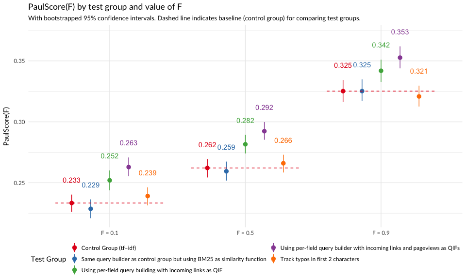
Figure 4: Average per-group PaulScore for various values of F (0.1, 0.5, and 0.9) with bootstrapped confidence intervals.
Engagement
In Figures 5 and 6, we see that the test groups that used BM25 with incoming links and pageviews as query-independent factors engaged with their search results more. The group whose search configuration included pageviews had a much higher clickthrough rate than the control group when they did not reformulate their search query.
engagement_overall <- searches %>%
  filter(results == "some") %>%
  group_by(`test group`) %>%
  summarize(clickthroughs = sum(clickthrough > 0),
            searches = n(), ctr = clickthroughs/searches) %>%
  ungroup
engagement_overall <- cbind(
  engagement_overall,
  as.data.frame(
    binom:::binom.bayes(
      engagement_overall$clickthroughs,
      n = engagement_overall$searches)[, c("mean", "lower", "upper")]
    )
  )
engagement_overall %>%
ggplot(aes(x = 1, y = mean, color = `test group`)) +
geom_hline(aes(yintercept = mean), linetype = "dashed", color = RColorBrewer::brewer.pal(3, "Set1")[1],
data = filter(engagement_overall, `test group` == "Control Group (tf–idf)")) +
geom_pointrange(aes(ymin = lower, ymax = upper), position = position_dodge(width = 1)) +
scale_color_brewer("Test Group", palette = "Set1", guide = guide_legend(ncol = 2)) +
scale_y_continuous(labels = scales::percent_format(), expand = c(0.01, 0.01)) +
labs(x = NULL, y = "Clickthrough rate",
title = "Engagement with search results by test group") +
geom_text(aes(label = sprintf("%.1f%%", 100 * ctr), y = upper + 0.0025, vjust = "bottom"),
position = position_dodge(width = 1)) +
theme_minimal(base_family = "Lato") +
theme(legend.position = "bottom")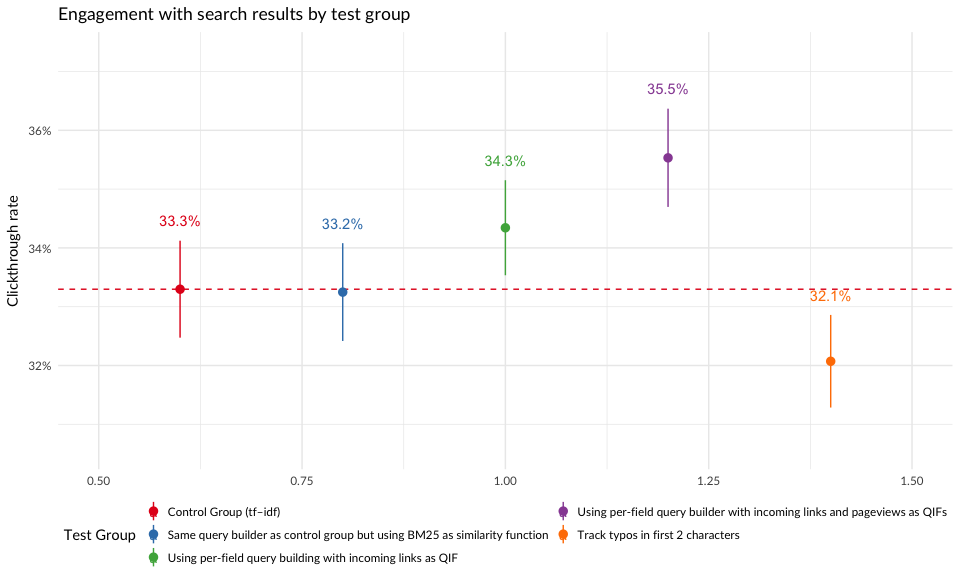
Figure 5: Clickthrough rates of test groups.
# Figure out engagement (clickthroughs) on a per-search ("query cluster") basis:
per_search_engagement <- query_reformulations %>%
  filter(results == "some") %>%
  group_by(`test group`, linkage,
           search = paste(search_id, cluster),
           reformulated = reformulations > 0) %>%
  summarize(clickthroughs = sum(clickthrough), `non-ZR searches` = n())

engagement <- per_search_engagement %>%
  group_by(`test group`, linkage,
           reformulated = ifelse(reformulated, "reformulated query", "did not reformulate query")) %>%
  summarize(clickthroughs = sum(clickthroughs > 0),
            searches = n(), ctr = clickthroughs/searches) %>%
  ungroup
engagement <- cbind(
  engagement,
  as.data.frame(
    binom:::binom.bayes(
      engagement$clickthroughs,
      n = engagement$searches)[, c("mean", "lower", "upper")]
    )
  )
engagement %>%
ggplot(aes(x = 1, y = mean, color = `test group`)) +
geom_hline(aes(yintercept = mean), linetype = "dashed", color = RColorBrewer::brewer.pal(3, "Set1")[1],
data = filter(engagement, `test group` == "Control Group (tf–idf)")) +
geom_pointrange(aes(ymin = lower, ymax = upper), position = position_dodge(width = 1)) +
facet_grid(reformulated ~ linkage, scales = "free_y") +
scale_color_brewer("Test Group", palette = "Set1", guide = guide_legend(ncol = 2)) +
scale_y_continuous(labels = scales::percent_format(), expand = c(0.01, 0.01)) +
labs(x = NULL, y = "Clickthrough rate",
title = "Engagement with search results by test group and presence of query reformulation",
subtitle = "Queries were grouped via hierarchical clustering using average/complete/single linkage and edit distance adjusted by search results in common") +
geom_text(aes(label = sprintf("%.1f%%", 100 * ctr), y = upper + 0.005, vjust = "bottom"),
position = position_dodge(width = 1)) +
theme_minimal(base_family = "Lato") +
theme(legend.position = "bottom",
panel.grid.major.x = element_blank(),
panel.grid.minor.x = element_blank(),
axis.ticks.x = element_blank(),
axis.text.x = element_blank(),
strip.background = element_rect(fill = "gray90"),
panel.border = element_rect(color = "gray30", fill = NA))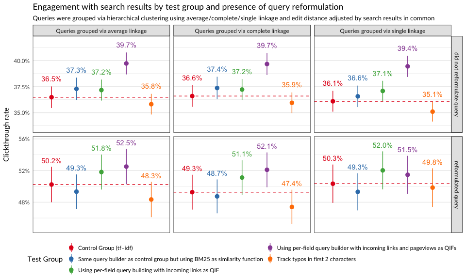
Figure 6: Clickthrough rates of test groups after splitting searches into those having query reformulations and those without query reformulations.
First Clicked Result’s Position
In Figure 7, we see that users who got the “all-field” query builder with BM25 were much less likely to click on the first search result first than the other groups. Other test groups (whose search configurations used incoming links) first clicked on the first result at a much higher rate than users in the control group.
safe_ordinals <- function(x) {
  return(vapply(x, toOrdinal::toOrdinal, ""))
}
first_clicked <- searches %>%
  filter(results == "some" & clickthrough & !is.na(`first clicked result's position`)) %>%
  mutate(`first clicked result's position` = ifelse(`first clicked result's position` < 4, safe_ordinals(`first clicked result's position` + 1), "5th or higher")) %>%
  group_by(`test group`, `first clicked result's position`) %>%
  tally %>%
  mutate(total = sum(n), prop = n/total) %>%
  ungroup
set.seed(0)
temp <- as.data.frame(binom:::binom.bayes(first_clicked$n, n = first_clicked$total, tol = .Machine$double.eps^0.1)[, c("mean", "lower", "upper")])
first_clicked <- cbind(first_clicked, temp); rm(temp)
first_clicked %>%
ggplot(aes(x = 1, y = mean, color = `test group`)) +
geom_hline(
aes(yintercept = mean),
linetype = "dashed", color = RColorBrewer::brewer.pal(3, "Set1")[1],
data = filter(first_clicked, `test group` == "Control Group (tf–idf)")
) +
geom_pointrange(aes(ymin = lower, ymax = upper), position = position_dodge(width = 1)) +
geom_text(aes(label = sprintf("%.1f", 100 * prop), y = upper + 0.0025, vjust = "bottom"),
position = position_dodge(width = 1)) +
scale_y_continuous(labels = scales::percent_format(),
expand = c(0, 0.005), breaks = seq(0, 1, 0.01)) +
scale_color_brewer("Test Group", palette = "Set1", guide = guide_legend(ncol = 2)) +
facet_wrap(~ `first clicked result's position`, scale = "free_y", nrow = 1) +
labs(x = NULL, y = "Proportion of searches",
title = "Position of the first clicked result",
subtitle = "With 95% credible intervals") +
theme_minimal(base_family = "Lato") +
theme(legend.position = "bottom",
panel.grid.major.x = element_blank(),
panel.grid.minor.x = element_blank(),
axis.ticks.x = element_blank(),
axis.text.x = element_blank(),
strip.background = element_rect(fill = "gray90"),
panel.border = element_rect(color = "gray30", fill = NA))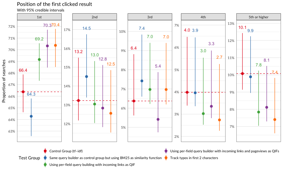
Figure 7: First clicked result’s position by group.
Conclusion
We recommend switching to BM25 ranking with incoming links (and possibly pageviews) as query-independent factors, as this configuration appears to give users results that are more relevant and that they engage with more (especially the first search result).
References
Software
- R Core Team (2016). R: A Language and Environment for StatisticalComputing. R Foundation for Statistical Computing, Vienna,Austria. https://www.R-project.org/
- Bache SM and Wickham H (2014). magrittr: A Forward-Pipe Operatorfor R. R package version 1.5, https://CRAN.R-project.org/package=magrittr
- Wickham H (2009). ggplot2: Elegant Graphics for Data Analysis.Springer-Verlag New York. ISBN 978-0-387-98140-6, http://ggplot2.org
- Wickham H and Francois R (2016). dplyr: A Grammar of DataManipulation. R package version 0.5.0, https://CRAN.R-project.org/package=dplyr
-
Wickham H (2016). tidyr: Easily Tidy Data with
spread()andgather()Functions. R package version 0.6.0, https://CRAN.R-project.org/package=tidyr - Wickham H, Hester J and Francois R (2016). readr: Read TabularData. R package version 1.0.0, https://CRAN.R-project.org/package=readr
- Dorai-Raj S (2014). binom: Binomial Confidence Intervals ForSeveral Parameterizations. R package version 1.1-1, https://CRAN.R-project.org/package=binom
- Allaire J, Cheng J, Xie Y, McPherson J, Chang W, Allen J, WickhamH, Atkins A and Hyndman R (2016). rmarkdown: Dynamic Documentsfor R. R package version 1.1, https://CRAN.R-project.org/package=rmarkdown
- Xie Y (2016). knitr: A General-Purpose Package for Dynamic ReportGeneration in R. R package version 1.14, http://yihui.name/knitr/
- Xie Y (2015). Dynamic Documents with R and knitr, 2nd edition.Chapman and Hall/CRC, Boca Raton, Florida. ISBN 978-1498716963, http://yihui.name/knitr/
- Xie Y (2014). “knitr: A Comprehensive Tool for ReproducibleResearch in R.” In Stodden V, Leisch F and Peng RD (eds.),Implementing Reproducible Computational Research. Chapman andHall/CRC. ISBN 978-1466561595, http://www.crcpress.com/product/isbn/9781466561595