Second Test Of Cross-wiki Search
Helping More Users Discover Content On Wikipedia’s Sister Projects
Erik Bernhardson
Senior Software Engineer, Wikimedia FoundationJan Drewniak
User Experience Engineer, Wikimedia FoundationDan Garry
Product Manager (Search Backend), Wikimedia FoundationMikhail Popov
Data Analyst, Wikimedia FoundationDeb Tankersley
Product Manager (Analysis, Search Frontend), Wikimedia Foundation24 April 2017
Abstract
Discovery’s Frontend and Backend Search teams ran an A/B test from 17 March 2017 to 27 March 2017 to assess the effectiveness of performing cross-wiki searches and showing results from sister projects (such as Wikisource and Wikiquote) to randomly selected users on Arabic, Catalan, French, German, Italian, Persian, Polish, and Russian Wikipedias. We found that relatively few users clicked on the cross-wiki results and that overall engagement varied greatly across the wikis. For example, Test group users were more likely to engage with their (cross-wiki and same-wiki) search results than the Control group were with their (same-wiki only) results on Arabic and Polish Wikipedias; counter-intuitively, the opposite was true on German and Italian Wikipedias. Given that we did observe a positive difference in engagement in 5 out of 8 wikis, Analysis’s recommendation is to move forward with the cross-wiki search project. That is, there does not appear to be overwhelming evidence that we should not continue with the cross-wiki search project, and we are left to wonder if – perhaps – there are cultural differences at play, but this would require research (see Discussion).
{ RMarkdown Source | Analysis Codebase }
Introduction
Within the Wikimedia Foundation’s Engineering group, the Discovery department’s mission is to make the wealth of knowledge and content in the Wikimedia projects (such as Wikipedia) easily discoverable. The Search team is responsible for maintaining and enhancing the search features and APIs for MediaWiki, such as language detection – i.e. if a French Wikipedia visitor searches and gets fewer than 3 results, we check if maybe their query is in another language, and if our language detection determines that the query’s language is most likely German (for example), then in addition to results from French Wikipedia, they would also get results from German Wikipedia, if any.
Specifically, the Search team’s current goal is to add cross-wiki searching – that is, providing search results from other (also referred to as “sister”) Wikimedia projects (“wikis”) within the same language. For example, if a work (e.g. a book or poem) on French Wikisource matched the user’s query, that user would be shown results from French Wikisource in addition to any results from French Wikipedia. In our previous report (2017), we showed that there was some evidence that suggested these additional “cross-wiki” search results helped user engagement but due to some issues with the user interface the results were not definitive, and so this test was meant to be a follow-up for us after we corrected those issues.
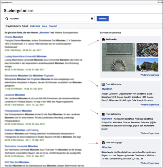
Figure 1: Example of cross-wiki search results on German Wikipedia, with sister wikis in the sidebar ordered according to recall. Multimedia results (including results from Wikimedia Commons) are shown first, regardless of the sidebar ordering.
For the users who received the experimental user experience (UX), each additional wiki’s top result was shown as a box in a sidebar with a link to view more results (see Figure 11). There was one group of users who received the experimental UX and one control group that did not:
- Control
- This group received the baseline user experience, which only includes the search results from the wiki they are on. To make their experience comparable to the test groups with respect to latency, we performed the search across the additional indices, but did not show the results to the end user.
- Test
- This group received the experimental user experience, which includes search results from other wikis (if any were returned). The boxes holding the results (one box for each wiki) were ordered according to recall – the volume of search results returned for each respective wiki.
The primary questions we wanted to answer are:
Did users who saw the additional cross-wiki results engage with those results?
Was the overall engagement with search results better or worse compared to the controls?
On 17 March 2017 we deployed an A/B test on the desktop version of Arabic, Catalan, French, German, Italian, Persian, Polish, and Russian Wikipedias to assess the efficacy of this feature. The test concluded on 27 March 2017, after a total of 42178 search sessions had been anonymously tracked.
Methods
This test’s event logging (EL) was implemented in JavaScript according to the TestSearchSatisfaction2 (TSS2) schema, which is the one used by the Search team for its metrics on desktop, data was stored in a MySQL database, and analyzed and reported using R (R Core Team 2016).
import::from(dplyr, group_by, ungroup, keep_where = filter, mutate, arrange, select, transmute, left_join, summarize, bind_rows, case_when, if_else, rename)
library(ggplot2)
Data
experiment_nodes <- c(
  "Wikipedia visitors on Desktop",
  "Arabic (1.21%)", "Catalan (0.23%)", "French (5.7%)", "German (7.18%)",
  "Italian (2.81%)", "Persian (0.57%)", "Polish (2.01%)", "Russian (6.6%)",
  "Other Languages (73.69%)",
  "In A/B Test", "In EL but not in test", "Not in Event Logging",
  "Test", "Control"
)
experiment_edges <- list(
  "Wikipedia visitors on Desktop" = list(
    "Arabic (1.21%)" = 0.012,
    "Catalan (0.23%)" = 0.002,
    "French (5.7%)" = 0.057,
    "German (7.18%)" = 0.072,
    "Italian (2.81%)" = 0.028,
    "Persian (0.57%)" = 0.006,
    "Polish (2.01%)" = 0.020,
    "Russian (6.6%)" = 0.066,
    "Other Languages (73.69%)" = 0.737
  ),
  "Other Languages (73.69%)" = list(
    "In EL but not in test" = 1/200,
    "Not in Event Logging" = 199/200
  ),
  "Arabic (1.21%)" = list(
    "Not in Event Logging" = 24/25,
    "In EL but not in test" = (1/25) * 7/8,
    "In A/B Test" = (1/25) * 1/8
  ),
  "Catalan (0.23%)" = list(
    "Not in Event Logging" = 5/6,
    "In EL but not in test" = (1/6) * 33/34,
    "In A/B Test" = (1/6) * 1/34
  ),
  "French (5.7%)" = list(
    "Not in Event Logging" = 69/70,
    "In EL but not in test" = (1/70) * 2/3,
    "In A/B Test" = (1/70) * 1/3
  ),
  "German (7.18%)" = list(
    "Not in Event Logging" = 107/108,
    "In EL but not in test" = (1/108) * 1/2,
    "In A/B Test" = (1/108) * 1/2
  ),
  "Italian (2.81%)" = list(
    "Not in Event Logging" = 41/42,
    "In EL but not in test" = (1/42) * 4/5,
    "In A/B Test" = (1/42) * 1/5
  ),
  "Persian (0.57%)" = list(
    "Not in Event Logging" = 7/8,
    "In EL but not in test" = (1/8) * 24/25,
    "In A/B Test" = (1/8) * 1/25
  ),
  "Polish (2.01%)" = list(
    "Not in Event Logging" = 34/35,
    "In EL but not in test" = (1/35) * 5/6,
    "In A/B Test" = (1/35) * 1/6
  ),
  "Russian (6.6%)" = list(
    "Not in Event Logging" = 70/71,
    "In EL but not in test" = (1/71) * 2/3,
    "In A/B Test" = (1/71) * 1/3
  ),
  "In A/B Test" = list("Control" = 1/2, "Test" = 1/2)
)
The data was collected according to the TSS2 schema, revision 16270835. Figure 2 shows the flow of Wikipedia visitors on Desktop. Approximately 26.3%2 of the unique desktop devices that visit the 2703 Wikipedias are accounted for by the 8 languages. In general, desktop users are randomly selected for anonymous tracking at a rate of 1 in 200, but for 8 wikis we changed the sampling rates to those shown in Table 14.
| Language | Chance of getting selected for EL | Chance of getting into A/B Test* | |
|---|---|---|---|
| arwiki | Arabic | 1 in 25 | 1 in 8 |
| cawiki | Catalan | 1 in 6 | 1 in 34 |
| frwiki | French | 1 in 70 | 1 in 3 |
| dewiki | German | 1 in 108 | 1 in 2 |
| itwiki | Italian | 1 in 42 | 1 in 5 |
| fawiki | Persian | 1 in 8 | 1 in 25 |
| plwiki | Polish | 1 in 35 | 1 in 6 |
| ruwiki | Russian | 1 in 71 | 1 in 3 |
Users who made it into the test were then randomly assigned to one of the two groups described above: Control and Test.
ds <- riverplot::default.style(); ds$col <- "gray"; ds$srt <- 30
visitor_flow <- riverplot::makeRiver(
  experiment_nodes, experiment_edges,
  node_xpos = c(1, 2, 2, 2, 2, 2, 2, 2, 2, 2, 3, 3, 3, 4, 4),
  node_styles = list(
    "Wikipedia visitors on Desktop" = list(col = "orange"),
    "Arabic (1.21%)" = list(col = "orange"),
    "Catalan (0.23%)" = list(col = "orange"),
    "French (5.7%)" = list(col = "orange"),
    "German (7.18%)" = list(col = "orange"),
    "Italian (2.81%)" = list(col = "orange"),
    "Persian (0.57%)" = list(col = "orange"),
    "Polish (2.01%)" = list(col = "orange"),
    "Russian (6.6%)" = list(col = "orange"),
    "In A/B Test" = list(col = "orange"),
    "Control" = list(col = RColorBrewer::brewer.pal(3, "Set1")[1]),
    "Test" = list(col = RColorBrewer::brewer.pal(3, "Set1")[2])
  )
)
x <- plot(visitor_flow, node_margin = 3, default_style = ds, fix.pdf = TRUE)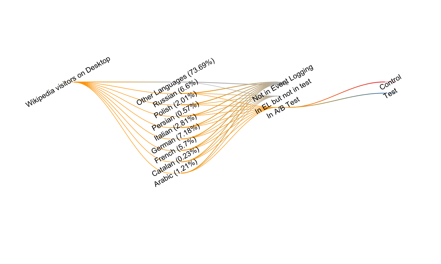
Figure 2: Flow of Wikipedia visitors into the A/B test.
We would like to note that our event logging does not support cross-wiki tracking, so after the user leaves the search results page, we cannot tell whether they have performed subsequent searches, nor how or how long the user engaged with the visited result’s page. See Phabricator ticket T160004 for full details of the implementation on both back-end and front-end.
Results
After the test has concluded on 27 March 2017, we processed the collected data and filtered out duplicated events, extraneous search engine result pages (SERPs), and kept only the searches for which we had both event logging (EL) data and logs of searches (Cirrus requests). This left us with a total of 42278 search sessions (see Table 2 for the full breakdown by wiki and group). Table 3 breaks down the counts of clicks on same-wiki results (e.g. a Italian Wikipedia visitor clicking on a Italian Wikipedia article) and clicks on sister-projects results (e.g. an Italian Wikipedia visitor clicking on an Italian Wikinews article).
session_counts <- searches %>%
  group_by(Wiki = wiki, group) %>%
  summarize(sessions = length(unique(session_id))) %>%
  xtabs(sessions ~ Wiki + group, data = .) %>%
addmargins| Control | Test | Both | |
|---|---|---|---|
| Arabic Wikipedia | 2144 | 2216 | 4360 |
| Catalan Wikipedia | 2970 | 2892 | 5862 |
| French Wikipedia | 2624 | 2679 | 5303 |
| German Wikipedia | 2641 | 2757 | 5398 |
| Italian Wikipedia | 2842 | 2781 | 5623 |
| Persian Wikipedia | 2389 | 2368 | 4757 |
| Polish Wikipedia | 2513 | 2505 | 5018 |
| Russian Wikipedia | 2952 | 3005 | 5957 |
| All 8 wikis | 21075 | 21203 | 42278 |
click_counts <- searches %>%
  keep_where(event != "SERP") %>%
  group_by(Group = group, event) %>%
  dplyr::count() %>%
  xtabs(n ~ Group + event, data = .) %>%
addmargins| Same-wiki clicks | Sister-project clicks | Textcat clicks | Overall clicks | |
|---|---|---|---|---|
| Control | 12999 | 0 | 1 | 13000 |
| Test | 12019 | 478 | 2 | 12499 |
| Both | 25018 | 478 | 3 | 25499 |
Zero Results Rate (ZRR)
The zero results rate (ZRR) – proportion of searches yielding zero results – is one of Discovery’s Search Team’s key performance indicators (KPIs), and we are always interested in lowering that number (but not at the expense of results’ relevance). While we were primarily interested in searchers’ engagement with the search result for this test, we included this section as a consistency check – that the zero results rate is lower when a cross-wiki search is performed (see Figure 3).
zrr <- searches %>%
  group_by(wiki, group, serp_id) %>%
  summarize(
    same = any(`cirrus log: some same-wiki results`),
    sister = any(`cirrus log: some sister-wiki results`),
    either = same || sister
  ) %>%
  summarize(
    total_searches = n(),
    `ZRR when counting just same-wiki results` = sum(!same),
    `ZRR when including sister-wiki results` = sum(!either)
  ) %>%
  ungroup %>%
  tidyr::gather(results, zr_searches, -c(wiki, group, total_searches)) %>%
  group_by(wiki, group, results) %>%
  dplyr::do(binom::binom.bayes(.$zr_searches, .$total_searches, conf.level = 0.95))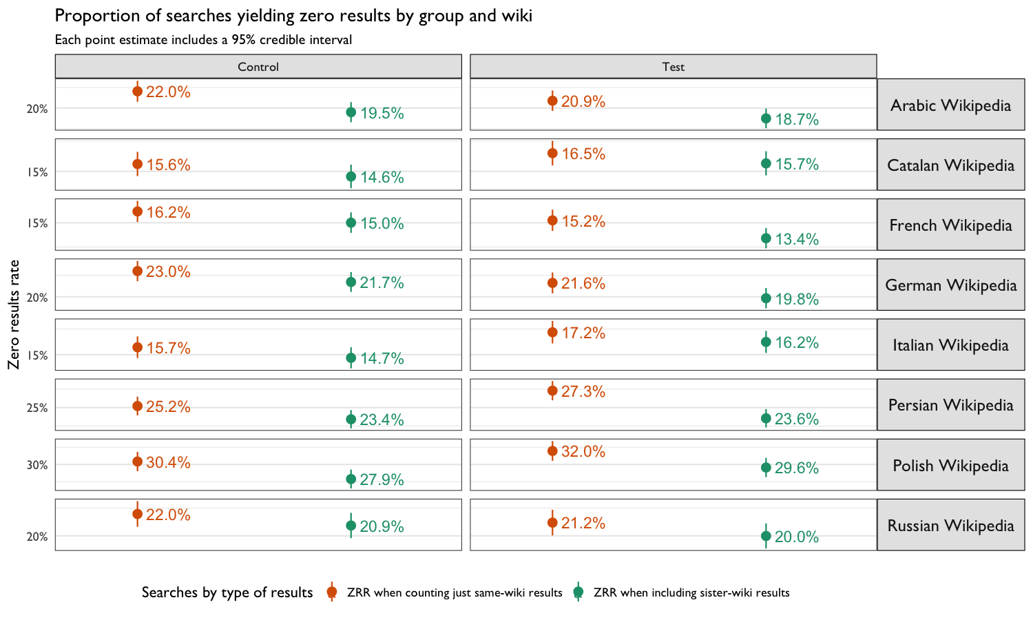
Figure 3: Proportion of searches yielding zero results broken up by group, wiki, and type of results (same-wiki only vs. including cross-wiki results).
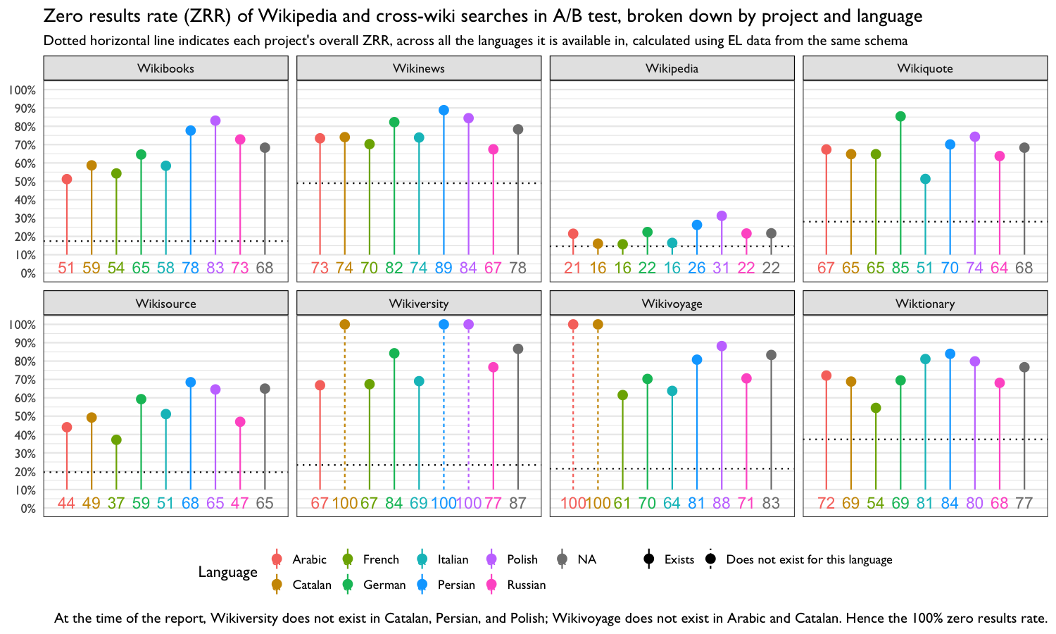
Figure 4: The proportion of searches that yielded zero results was the lowest for Wikipedia and Wikisource, with the other projects having very high zero result rates. The ZRR was calculated using back-end search logs, which included searches from controls. To control for lag, we performed cross-wiki searches for everyone in the A/B test, regardless of group membership.
In Figure 4, we broke the ZRR from Figure 3 down by language and project and included a reference marker for each project’s overall ZRR (aggregated across all the languages the project is available in). Almost all of the projects are available (at the time of the test and at the time of writing this report) in Arabic, Catalan, French, German, Italian, Persian, Polish, and Russian. Of particular note are the overall ZRR of projects like Wikinews and Wiktionary (both exist in Catalan, Italian, Persian, and Polish), which appear to be much lower than the ZRR observed in this test.
In fact, the ZRR in these eight languages is much higher than the overall ZRR for every project. We suspect this is partly responsible for the low sister-project click counts seen in Table 3. This supports our previous intuition that people search differently on different projects and that people sometimes tailor their searches to the project they are on. For example, searching for “Barack Obama birthdate” or “Fast and Furious movies” on Wikipedia simply does not make a whole lot of sense on other projects such as Wiktionary and Wikivoyage.
Engagement
We used the clickthrough rate as an indicator of users’ engagement with search results and as a measure of the results’ relevance. That is, if we present users with more relevant results (such as those from Wikipedia’s sister projects), then we expect the clickthrough rate to be higher in the test group compared to that of controls. Figure 5 shows that various search activity measures did not vary too much from one group to another.
counts <- searches %>%
  group_by(wiki, group, session_id) %>%
  summarize(searches = length(unique(serp_id)),
            SERPs = sum(event == "SERP")) %>%
  summarize(`searches\nper session` = mean(searches),
            `SERPs seen\n per session` = mean(SERPs)) %>%
  ungroup %>%
  tidyr::gather(metric, value, -c(wiki, group))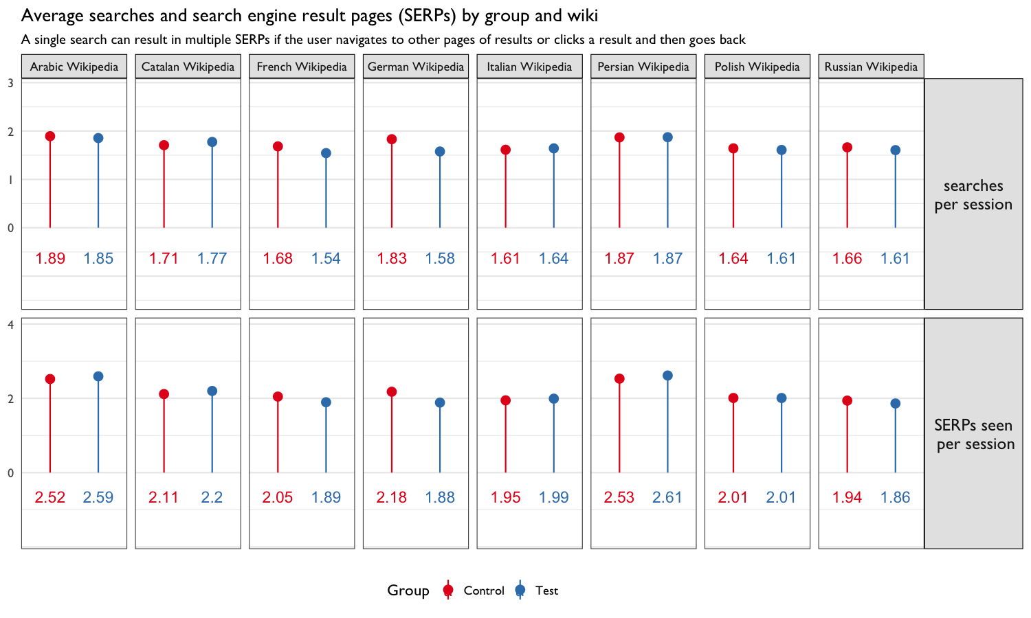
Figure 5: Average number of searches, average number of search engine result pages (SERPs), total searches, total SERPs, and total sessions by group and wiki. The groups did not appear to behave too differently. For example, the two groups had very similar average searches per user.
searches_H1 <- searches %>%
  group_by(serp_id) %>%
  keep_where(
    `cirrus log: some same-wiki results` &
      `cirrus log: some sister-wiki results`
  ) %>%
  select(serp_id) %>%
  ungroup %>%
  arrange(serp_id) %>%
  dplyr::distinct() %>%
  dplyr::left_join(searches, by = "serp_id") %>%
  group_by(wiki, group, serp_id) %>%
  summarize(clickthrough = any(event != "SERP")) %>%
  summarize(searches = n(), clickthroughs = sum(clickthrough)) %>%
  group_by(wiki, group) %>%
  dplyr::do(binom::binom.bayes(.$clickthroughs, .$searches, conf.level = 0.95))
searches_H2 <- searches %>%
  group_by(serp_id) %>%
  keep_where(
    `cirrus log: some same-wiki results` &
      `cirrus log: some sister-wiki results`
  ) %>%
  select(serp_id) %>%
  ungroup %>%
  arrange(serp_id) %>%
  dplyr::distinct() %>%
  dplyr::left_join(searches, by = "serp_id") %>%
  group_by(date, wiki, group, serp_id) %>%
  summarize(clickthrough = any(event != "SERP")) %>%
  summarize(searches = n(), clickthroughs = sum(clickthrough)) %>%
  group_by(date, wiki, group) %>%
  dplyr::do(binom::binom.bayes(.$clickthroughs, .$searches, conf.level = 0.95))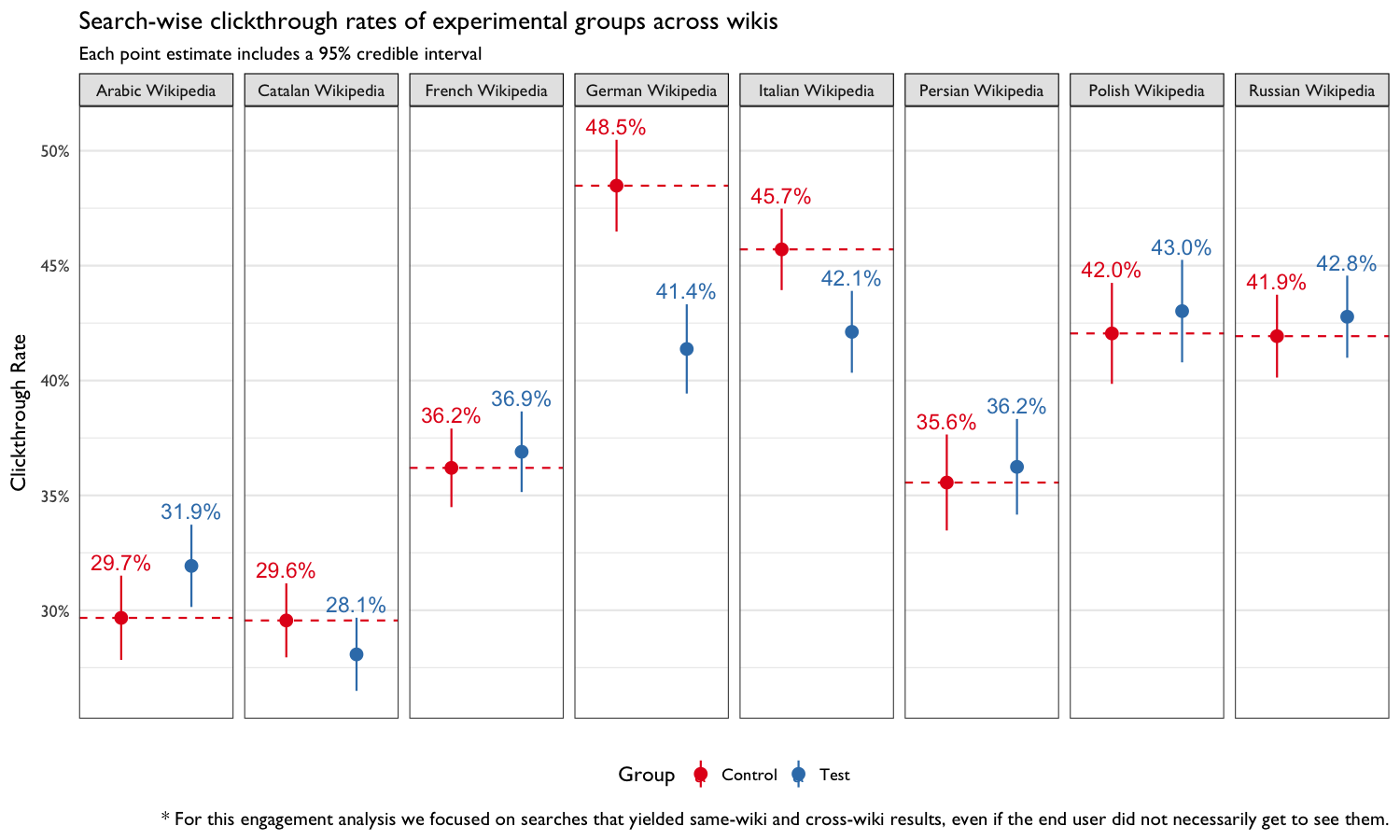
Figure 6: Clickthrough rates of experimental groups, split by wiki.
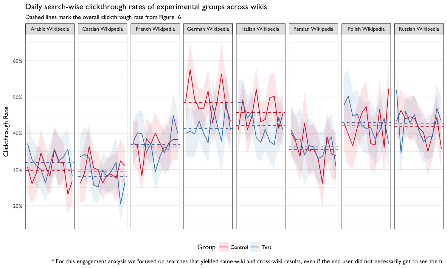
Figure 7: Day-by-day clickthrough rates of experimental groups, split by wiki.
bcda_H1 <- searches_H1 %>%
  arrange(wiki, desc(group)) %>%
  group_by(wiki) %>%
  dplyr::do(BCDA::tidy(BCDA::beta_binom(.$x, .$n), interval_type = "HPD")) %>%
  ungroup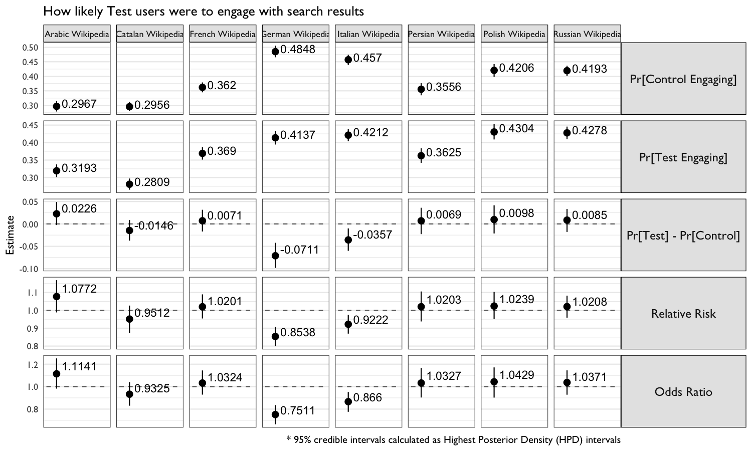
Figure 8: By-wiki comparison of the Control group’s probability of engaging with results to the Test group’s probability.
| Wiki | Relative Risk | 95% CI |
|---|---|---|
| Arabic Wikipedia | 1.077 | (0.988, 1.168) |
| Catalan Wikipedia | 0.951 | (0.874, 1.027) |
| French Wikipedia | 1.020 | (0.954, 1.089) |
| German Wikipedia | 0.854 | (0.800, 0.908) |
| Italian Wikipedia | 0.922 | (0.870, 0.975) |
| Persian Wikipedia | 1.020 | (0.938, 1.105) |
| Polish Wikipedia | 1.024 | (0.951, 1.103) |
| Russian Wikipedia | 1.021 | (0.959, 1.082) |
In Figures 6, 7, and 8, we see that engagement was higher in Test than in Control on 5 of the 8 wikis (Arabic, French, Persian, Polish, and Russian Wikipedias) but lower on the other 4 (Italian, Catalan, and most drastically German Wikipedias).
Table 4 shows the relative risk – how much more likely each respective test group is to engage with the search results (same-wiki or cross-wiki) than the Control group. For example, on Catalan Wikipedia, users in the Test are 0.951 times more likely to click on a result than users in the Control group. While most of the estimates are greater than 1 (suggesting more relevant results), the 95% credible intervals contain 1, meaning we do not have sufficient evidence to draw definitive conclusions.
indices_subset <- indices %>%
  keep_where(!(project %in% c("wikipedia"))) %>%
  group_by(cirrus_id) %>%
  summarize(sisters = length(unique(project[n_results > 0])))
sister_ctr <- searches %>%
  keep_where(group != "Control") %>%
  dplyr::inner_join(indices_subset, by = "cirrus_id") %>%
  group_by(group, wiki, cirrus_id) %>%
  summarize(
    `clicks (sister project)` = sum(event == "sister-project click"),
    sisters = sisters[1]
  ) %>%
  ungroup %>%
  mutate(
    `clicks (sister project)` = dplyr::case_when(
      .$`clicks (sister project)` == 0 ~ "0",
      .$`clicks (sister project)` == 1 ~ "1",
      .$`clicks (sister project)` > 1 ~ "2+"
    ),
    sisters = dplyr::case_when(
      .$sisters == 0 ~ "0",
      .$sisters == 1 ~ "1",
      .$sisters == 2 ~ "2",
      .$sisters > 2 ~ "3+"
    ),
    invalid = (`clicks (sister project)` %in% c("1", "2+")) & (sisters == "0")
  ) %>%
  keep_where(!invalid) %>%
  select(-invalid) %>%
  group_by(`clicks (sister project)`, sisters) %>%
  dplyr::count() %>%
  ungroup %>%
xtabs(n ~ sisters + `clicks (sister project)`, data = .)| 0 cross-wiki clicks | 1 cross-wiki click | 2+ cross-wiki clicks | |
|---|---|---|---|
| 0 sister projects | 14039 | 0 | 0 |
| 1 sister projects | 5192 | 90 | 17 |
| 2 sister projects | 3679 | 64 | 7 |
| 3+ sister projects | 12270 | 154 | 32 |
BF <- LearnBayes::ctable(sister_ctr, matrix(rep(1, nrow(sister_ctr)*ncol(sister_ctr)), nrow(sister_ctr)))
BCCT.fit <- sister_ctr %>%
  as.data.frame() %>%
  set_colnames(c("sisters", "clicks", "searches")) %>%
  conting::bcct(searches ~ sisters + clicks + sisters:clicks, data = .,
                n.sample = 2e4, prior = "UIP")
BCCT.summary <- summary(BCCT.fit, n.burnin = 1e3, thin = 5)
BCCT.estimates <- as.data.frame(BCCT.summary$int_stats[c("term", "post_mean", "lower", "upper")])
BCCT.estimates %>%
  mutate(
    term = sub("(Intercept)", "0 sister projects and 0 cross-wiki clicks", term, fixed = TRUE),
    term = sub(":", " and ", term, fixed = TRUE),
    term = sub("sisters1", "1 sister project", term, fixed = TRUE),
    term = sub("sisters2", "2 sister projects", term, fixed = TRUE),
    term = sub("sisters3", "3+ sister projects", term, fixed = TRUE),
    term = sub("clicks1", "1 cross-wiki click", term, fixed = TRUE),
    term = sub("clicks2", "2+ cross-wiki clicks", term, fixed = TRUE),
    ci = sprintf("(%.2f, %.2f)", lower, upper)
  ) %>%
  rename(Coefficient = term, Estimate = post_mean, `95% HPDI` = ci) %>%
  select(-c(lower, upper)) %>%
fable(format_caption(table_caps, "Log-linear Model"))| Coefficient | Estimate | 95% HPDI |
|---|---|---|
| 0 sister projects and 0 cross-wiki clicks | 4.532 | (4.13, 4.89) |
| 1 sister project | -2.413 | (-3.53, -1.35) |
| 2 sister projects | 0.751 | (0.34, 1.16) |
| 3+ sister projects | 0.226 | (-0.17, 0.67) |
| 1 cross-wiki click | 4.400 | (4.04, 4.80) |
| 2+ cross-wiki clicks | -1.530 | (-2.10, -1.02) |
| 1 sister project and 1 cross-wiki click | 3.030 | (1.97, 4.16) |
| 2 sister projects and 1 cross-wiki click | -1.128 | (-1.50, -0.68) |
| 3+ sister projects and 1 cross-wiki click | -0.949 | (-1.37, -0.51) |
| 1 sister project and 2+ cross-wiki clicks | -2.261 | (-3.75, -0.72) |
| 2 sister projects and 2+ cross-wiki clicks | 0.739 | (0.20, 1.25) |
| 3+ sister projects and 2+ cross-wiki clicks | 0.931 | (0.38, 1.56) |
Under the \(\chi^2\) discrepancy statistic, the Bayesian p value of 0.525 does not indicate that the interaction model is inadequate. Furthermore, Kass and Raftery (1995) suggest that \(2~\log_e(\mathrm{Bayes Factor}) = 301.608\) is very strong evidence against null hypothesis of independence. This means there is evidence of a relationship between number of projects displayed and number of clicks on those sister-wiki results.
Table 6 summarizes the Markov chain Monte Carlo (MCMC) results of fitting a Bayesian log-linear model to the data in Table 5. It suggests there is a strong interaction between number of projects returned and number of clicks on those projects. Contrasting the negative estimate for “3+ sister projects and 1 cross-wiki click” (-0.949) to the positive estimates for “2/3+ sister projects and 2+ cross-wiki clicks” (0.739 and 0.931, respectively, with the lower bounds of both HPD intervals being greater than zero), the model strongly suggests the relationship is positive – that more sister projects shown to the user yields more cross-wiki clicks, up to a point.
single_clicks <- searches %>%
  keep_where(group != "Control", `cirrus log: some sister-wiki results`, `cirrus log: some same-wiki results`) %>%
  group_by(serp_id) %>%
  summarize(
    clicks = sum(event != "SERP"),
    `clicks (sister project)` = sum(event == "sister-project click")
  ) %>%
  keep_where(clicks == 1) %>%
  group_by(`clicks (sister project)`) %>%
  dplyr::count() %>%
  xtabs(n ~ `clicks (sister project)`, data = .)
Of the 394 unique searches that included a click on the cross-wiki results, 232 were searches where the user received both sets of results (same-wiki and cross-wiki) but clicked only once and specifically on a cross-wiki result. This suggests that for some users the results from sister projects may have been more relevant than the results from the wiki they were on.
Discussion
We are not actually sure why there is such a drastic negative difference between the two groups on German Wikipedia since we are not actually removing any search results, and we would expect users to at least have an engagement rate in the same ballpark, and it is interesting to see a similar negative difference on Italian Wikipedia also. From a technical implementation perspective, there should not have been anything particular about those two wikis that impacted event logging or display of results. Perhaps there is a cultural difference in task/intent – such that when users saw previews of results from the other projects, perhaps they learned what they wanted to learn, and with their curiosity satisfied, did not feel the need to click on any results – but that would require considerable human-computer interaction research to confirm or reject.
We also suspect that the high zero results rate for each of the sister projects for these languages may have been responsible for the few sister-project clicks. As shown in Table 6 in the Engagement analysis, there is evidence that suggests a positive relationship between number of sister projects in the sidebar and clicks on those cross-wiki results.
Acknowledgements
Finally, we would like to thank our colleagues Trey Jones (Software Engineer, Wikimedia Foundation) and Chelsy Xie (Data Analyst, Wikimedia Foundation) for their reviews of and feedback on this report.
References
Albert, Jim. 2014. LearnBayes: Functions for Learning Bayesian Inference. https://CRAN.R-project.org/package=LearnBayes.
Allaire, JJ, Joe Cheng, Yihui Xie, Jonathan McPherson, Winston Chang, Jeff Allen, Hadley Wickham, Aron Atkins, Rob Hyndman, and Ruben Arslan. 2016. Rmarkdown: Dynamic Documents for R. http://rmarkdown.rstudio.com.
Bache, Stefan Milton, and Hadley Wickham. 2014. Magrittr: A Forward-Pipe Operator for R. https://CRAN.R-project.org/package=magrittr.
Bernhardson, Erik, Jan Drewniak, Dan Garry, Mikhail Popov, and Deb Tankersley. 2017. A Test of Cross-Wiki Search: Helping Users Discover Content on Wikipedia’s Sister Projects. https://commons.wikimedia.org/wiki/File:A_Test_Of_Cross-wiki_Search_-_Helping_Users_Discover_Content_On_Wikipedia%E2%80%99s_Sister_Projects.pdf.
Dorai-Raj, Sundar. 2014. Binom: Binomial Confidence Intervals for Several Parameterizations. https://CRAN.R-project.org/package=binom.
Kass, R E, and Adrian E Raftery. 1995. “Bayes factors.” Journal of the American Statistical Association.
Keyes, Oliver, and Mikhail Popov. 2017. Wmf: R Code for Wikimedia Foundation Internal Usage. https://phabricator.wikimedia.org/diffusion/1821/.
Overstall, Antony M. 2016. Conting: Bayesian Analysis of Contingency Tables. https://CRAN.R-project.org/package=conting.
Popov, Mikhail. n.d. BCDA: Tools for Bayesian Categorical Data Analysis. https://github.com/bearloga/BCDA.
R Core Team. 2016. R: A Language and Environment for Statistical Computing. Vienna, Austria: R Foundation for Statistical Computing. https://www.R-project.org/.
Wickham, Hadley. 2009. Ggplot2: Elegant Graphics for Data Analysis. Springer-Verlag New York. http://ggplot2.org.
———. 2017. Tidyr: Easily Tidy Data with ’Spread()’ and ’Gather()’ Functions. https://CRAN.R-project.org/package=tidyr.
Wickham, Hadley, and Romain Francois. 2016. Dplyr: A Grammar of Data Manipulation. https://CRAN.R-project.org/package=dplyr.
Screenshot by Deb Tankersley available on Wikimedia Commons, licensed under CC BY-SA 4.0.↩
Relative traffic was calculated using a combination of Wikidata Query Service (WDQS) and Wikimedia Analytics’ monthly unique devices API. See the workbook for implementation.↩
The languages Wikipedia is available in were counted by querying Wikidata with this SPARQL query.↩
To see the sampling configuration, refer to Gerrit change 343104.↩