Second BM25 A/B Test Analysis
Erik Bernhardson (Engineering)
David Causse (Engineering & Review)
Trey Jones (Engineering & Review)
Mikhail Popov (Review)
Deb Tankersley (Product Management)
Chelsy Xie (Analysis & Report)
06 January 2017
{ RMarkdown Source | Analysis Codebase | PDF Version }
Executive Summary
In order to assess the efficacy of BM25 in space-less language, Discovery’s Search team has decided to conduct a second A/B test in Chinese, Japanese and Thai Wikipedias. We observed that the test group that used per-field query builder with incoming links and pageviews as query-independent factors had a much better Zero Result Rate but slightly worse PaulScores, large decrease in clickthrough rate, and fewer users clicked on the first result first, which indicates that we are showing test group users worse results. However, longer dwell-time and fewer query reformulations show that test group users might actually like the results they are getting better than the control group in that respect. We recommend deploying BM25 for all wikis but not reindexing projects in space-less languages for now.
Background
To improve the relevancy of search results, Discovery’s Search team decided to try a new document-ranking function called Okapi BM25 (BM stands for Best Matching), and ran an A/B test from August 30 to September 10 to assess the efficacy of the proposed switch. The analysis showed that BM25 ranking with incoming links and pageviews as query-independent factors appears to give users results that are more relevant and that they engage with more.
However, we then realized that our analysis chain is sub-optimal for space-less language queries, which will break words on every characters for the plain field. Therefore, we ran a second A/B test for Chinese, Japanese and Thai Wikipedias to test whether the new per-field BM25 builder is sufficiently worse with those languages. We are primarily interested in:
- Zero results rate, the proportion of searches that yielded zero results (smaller is usually better)
- Users’ engagement with the search results, measured as the clickthrough rate (bigger is better)
- PaulScore, a metric of search results’ relevancy that relies on the position of the clicked result[s] (bigger is better); see PaulScore Definition for more details
- Query reformulation – one way to think about the strength of our search engine is how many times the user reformulates their query; if a user in the test group has to reformulate their query many more times to get the results they are interested in, then maybe the change is for the worse
- Dwell Time, the time (seconds) that users stayed on the pages they visited by clicking on the search results (bigger is better)
- Scroll – if users scroll on the visited page, they are more likely to engage with the contents
# Install packages used in the report:
install.packages(c("devtools", "tidyverse", "binom"))
devtools::install_github("hadley/ggplot2")
# ^ development version of ggplot2 includes subtitles
devtools::install_github("wikimedia/wikimedia-discovery-polloi")
# ^ for converting 100000 into 100K via polloi::compress()
# Load packages that we will be using in this report:
library(tidyverse) # for ggplot2, dplyr, tidyr, broom, etc.
library(binom) # for Bayesian confidence intervals of proportions# PaulScore Calculation
query_score <- function(positions, F) {
if (length(positions) == 1 || all(is.na(positions))) {
# no clicks were made
return(0)
} else {
positions <- positions[!is.na(positions)] # when operating on 'events' dataset, searchResultPage events won't have positions
return(sum(F^positions))
}
}
# Bootstrapping
bootstrap_mean <- function(x, m, seed = NULL) {
if (!is.null(seed)) {
set.seed(seed)
}
n <- length(x)
return(replicate(m, mean(x[sample.int(n, n, replace = TRUE)])))
}Data
# Import events fetched from MySQL
load(path("data/ab-test_bm25.RData"))
events <- events[!duplicated(events$event_id),]
events <- events %>%
  group_by(date, wiki, test_group, session_id, search_id) %>%
  filter("searchResultPage" %in% action) %>%
  ungroup %>% as.data.frame() # remove search_id without SERP asscociated
events$test_group <- factor(
  events$test_group,
  levels = c("bm25:control", "bm25:inclinks_pv"),
  labels = c("Control Group (tf–idf)", "Using per-field query builder with incoming links and pageviews as QIFs"))
cirrus <- readr::read_tsv(path("data/ab-test_bm25_cirrus-results.tsv.gz"), col_types = "cccc")
cirrus <- cirrus[!duplicated(cirrus),]
events <- left_join(events, cirrus, by = c("event_id", "page_id", "cirrus_id"))
rm(cirrus)
For Chinese Wikipedia (zhwiki) and Japanese Wikipedia (jawiki), users had a 1 in 16 chance of being selected for anonymous tracking according to our TestSearchSatisfaction2 #15922352 event logging schema. Those users who were randomly selected to have their sessions anonymously tracked then had a 12 in 13 chance of being selected for the BM25 test. For Thai Wikipedia (thwiki), users had a 1 in 5 chance of being selected for search satisfaction tracking and then had a 38 in 39 chance of being selected for the BM25 test due to fewer visitors to that particular project. The sampled sessions were evenly put into a control group (tf-idf) and a test group (using per-field query builder with incoming links and pageviews as QIFs); see the first BM25 test report for more details. The test was deployed on October 27th and ran for a week for zhwiki and jawiki, but until November 15th for thwiki specifically.
The full-text (as opposed to auto-complete) searching event logging data was extracted from the database using this script. We collected a total of 230.2K events from 36.1K unique sessions. See Table 1 for counts broken down by wiki and test group.
events_summary <- events %>%
  group_by(wiki, `Test group` = test_group) %>%
  summarize(`Search sessions` = length(unique(search_id)), `Events recorded` = n()) %>% ungroup %>%
  {
    rbind(., tibble(
      `wiki` = "All Wikis",
      `Test group` = "Total",
      `Search sessions` = sum(.$`Search sessions`),
      `Events recorded` = sum(.$`Events recorded`)
    ))
  } %>%
  mutate(`Search sessions` = prettyNum(`Search sessions`, big.mark = ","),
         `Events recorded` = prettyNum(`Events recorded`, big.mark = ","))
knitr::kable(events_summary, format = "markdown", align = c("l", "l", "r", "r"))| wiki | Test group | Search sessions | Events recorded |
|---|---|---|---|
| jawiki | Control Group (tf–idf) | 7,579 | 54,261 |
| jawiki | Using per-field query builder with incoming links and pageviews as QIFs | 7,610 | 59,808 |
| thwiki | Control Group (tf–idf) | 3,889 | 18,954 |
| thwiki | Using per-field query builder with incoming links and pageviews as QIFs | 4,055 | 21,217 |
| zhwiki | Control Group (tf–idf) | 6,510 | 37,561 |
| zhwiki | Using per-field query builder with incoming links and pageviews as QIFs | 6,478 | 38,382 |
| All Wikis | Total | 36,121 | 230,183 |
Table 1: Counts of sessions anonymously tracked and events collected during the second A/B test (Oct 27 - Nov 15).
An issue we noticed with the event logging is that when the user goes to the next page of search results or clicks the Back button after visiting a search result, a new page ID is generated for the search results page. The page ID is how we connect click events to search result page events. There is currently a Phabricator ticket (T146337) for addressing these issues. For this analysis, we de-duplicated by connecting search engine results page (searchResultPage) events that have the exact same search query, and then connected click events together based on the searchResultPage connectivity.
temp <- events %>%
  filter(action == "searchResultPage") %>%
  group_by(session_id, search_id, query) %>%
  mutate(new_page_id = min(page_id)) %>%
  ungroup %>%
  select(c(page_id, new_page_id)) %>%
  distinct
events <- left_join(events, temp, by = "page_id"); rm(temp)
events$new_page_id[is.na(events$new_page_id)] <- events$page_id[is.na(events$new_page_id)]
temp <- events %>%
  filter(action == "searchResultPage") %>%
  arrange(new_page_id, ts) %>%
  mutate(dupe = duplicated(new_page_id, fromLast = FALSE)) %>%
  select(c(event_id, dupe))
events <- left_join(events, temp, by = "event_id"); rm(temp)
events$dupe[events$action != "searchResultPage"] <- FALSE
events <- events[!events$dupe & !is.na(events$new_page_id), ] %>%
  select(-c(page_id, dupe)) %>%
  rename(page_id = new_page_id) %>%
  arrange(date, session_id, search_id, page_id, desc(action), ts)
# Summarize on a page-by-page basis for each SERP:
searches <- events %>%
group_by(wiki, `test group` = test_group, session_id, search_id, page_id) %>%
filter("searchResultPage" %in% action) %>% # filter out searches where we have clicks but not searchResultPage events
summarize(ts = ts[1], query = query[1],
results = ifelse(n_results_returned[1] > 0, "some", "zero"),
clickthrough = "click" %in% action,
`no. results clicked` = length(unique(position_clicked))-1,
`first clicked result's position` = ifelse(clickthrough, position_clicked[2], NA),
`result page IDs` = paste(unique(result_pids[!is.na(result_pids)]), collapse=','),
`Query score (F=0.1)` = query_score(position_clicked, 0.1),
`Query score (F=0.5)` = query_score(position_clicked, 0.5),
`Query score (F=0.9)` = query_score(position_clicked, 0.9)) %>%
arrange(ts)
searches$`result page IDs`[searches$`result page IDs`==""] <- NAAfter de-duplicating, we collapsed 213.4K (searchResultPage and click) events into 64.5K searches. See Table 2 for counts broken down by wiki and test group.
events_summary2 <- events %>%
  group_by(wiki, `Test group` = test_group) %>%
  summarize(`Search sessions` = length(unique(search_id)), `Events recorded` = n()) %>% ungroup %>%
  {
    rbind(., tibble(
      `wiki` = "All Wikis",
      `Test group` = "Total",
      `Search sessions` = sum(.$`Search sessions`),
      `Events recorded` = sum(.$`Events recorded`)
    ))
  } %>%
  mutate(`Search sessions` = prettyNum(`Search sessions`, big.mark = ","),
         `Events recorded` = prettyNum(`Events recorded`, big.mark = ","))
searches_summary <- searches %>%
  group_by(wiki, `Test group` = `test group`) %>%
  summarize(`Search sessions` = length(unique(search_id)), `Searches recorded` = n()) %>% ungroup %>%
  {
    rbind(., tibble(
      `wiki` = "All Wikis",
      `Test group` = "Total",
      `Search sessions` = sum(.$`Search sessions`),
      `Searches recorded` = sum(.$`Searches recorded`)
    ))
  } %>%
  mutate(`Search sessions` = prettyNum(`Search sessions`, big.mark = ","),
         `Searches recorded` = prettyNum(`Searches recorded`, big.mark = ","))
knitr::kable(inner_join(searches_summary, events_summary2, by=c("wiki", "Test group", "Search sessions")),
format = "markdown", align = c("l", "l", "r", "r", "r"))| wiki | Test group | Search sessions | Searches recorded | Events recorded |
|---|---|---|---|---|
| jawiki | Control Group (tf–idf) | 7,579 | 13,839 | 50,845 |
| jawiki | Using per-field query builder with incoming links and pageviews as QIFs | 7,610 | 13,982 | 56,097 |
| thwiki | Control Group (tf–idf) | 3,889 | 7,005 | 16,379 |
| thwiki | Using per-field query builder with incoming links and pageviews as QIFs | 4,055 | 7,086 | 18,481 |
| zhwiki | Control Group (tf–idf) | 6,510 | 11,450 | 35,262 |
| zhwiki | Using per-field query builder with incoming links and pageviews as QIFs | 6,478 | 11,173 | 36,373 |
| All Wikis | Total | 36,121 | 64,535 | 213,437 |
Table 2: After searchResultPage De-duplication, Counts of sessions anonymously tracked and events collected during the second A/B test (Oct 27 - Nov 15).
There are 22.1K visitPage events (When the user clicks a link in the results a visitPage event is created). See Table 3 for counts broken down by wiki and test group.
# Summarize on a page-by-page basis for each visitPage:
clickedResults <- events %>%
  group_by(wiki, `test group` = test_group, session_id, search_id, page_id) %>%
  filter("visitPage" %in% action) %>% #only checkin and visitPage action
  summarize(ts = ts[1],
            dwell_time=ifelse("checkin"%in% action, max(checkin, na.rm=T), 0),
            scroll=sum(scroll)>0) %>%
  arrange(ts)
clickedResults$dwell_time[is.na(clickedResults$dwell_time)] <- 0
clickedResults_summary <- clickedResults %>%
group_by(wiki, `Test group` = `test group`) %>%
summarize(`Visited pages` = length(unique(page_id))) %>% ungroup %>%
{
rbind(., tibble(
`wiki` = "All Wikis",
`Test group` = "Total",
`Visited pages` = sum(.$`Visited pages`)
))
} %>%
mutate(`Visited pages` = prettyNum(`Visited pages`, big.mark = ","))
knitr::kable(clickedResults_summary, format = "markdown", align = c("l", "l", "r", "r"))| wiki | Test group | Visited pages |
|---|---|---|
| jawiki | Control Group (tf–idf) | 5,431 |
| jawiki | Using per-field query builder with incoming links and pageviews as QIFs | 5,954 |
| thwiki | Control Group (tf–idf) | 1,554 |
| thwiki | Using per-field query builder with incoming links and pageviews as QIFs | 1,776 |
| zhwiki | Control Group (tf–idf) | 3,591 |
| zhwiki | Using per-field query builder with incoming links and pageviews as QIFs | 3,807 |
| All Wikis | Total | 22,113 |
Table 3: Counts of visited pages from search sessions anonymously tracked during the second A/B test (Oct 27 - Nov 15).
Results
Zero Results Rate
In Figure 1, we see that the test group that used BM25 with incoming links and pageviews as query-independent factors had a significantly lower zero results rate (ZRR). Smaller ZRR is usually better, but looking at the PaulScore, engagement and First Clicked Result’s Position, we doubt that it came at the cost of relevance and engagement with the results. Figure 2 shows that zhwiki had the largest ZRR difference between control and test group.
zrr_pages <- searches %>%
  group_by(`test group`, results) %>%
  tally %>%
  spread(results, n) %>%
  mutate(`zero results rate` = zero/(some + zero)) %>%
  ungroup
zrr_pages <- cbind(zrr_pages, as.data.frame(binom:::binom.bayes(zrr_pages$zero, n = zrr_pages$some + zrr_pages$zero)[, c("mean", "lower", "upper")]))
zrr_pages %>%
ggplot(aes(x = `test group`, y = `mean`, color = `test group`)) +
geom_pointrange(aes(ymin = lower, ymax = upper)) +
scale_x_discrete(limits = levels(events$test_group)) +
scale_y_continuous(labels = scales::percent_format()) +
scale_color_brewer("Test Group", palette = "Set1", guide = FALSE) +
labs(x = NULL, y = "Zero Results Rate",
title = "Proportion of searches that did not yield any results, by test group",
subtitle = "With 95% credible intervals.") +
geom_text(aes(label = sprintf("%.2f%%", 100 * `zero results rate`),
vjust = "bottom", hjust = "center"), nudge_x = 0.1) 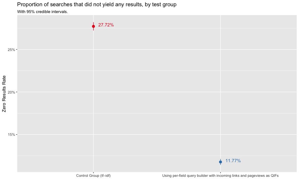
Figure 1: Zero results rate is the proportion of searches in which the user received zero results. Broken down by test group.
zrr_pages <- searches %>%
  group_by(wiki, `test group`, results) %>%
  tally %>%
  spread(results, n) %>%
  mutate(`zero results rate` = zero/(some + zero)) %>%
  ungroup
zrr_pages <- cbind(zrr_pages, as.data.frame(binom:::binom.bayes(zrr_pages$zero, n = zrr_pages$some + zrr_pages$zero)[, c("mean", "lower", "upper")]))
zrr_pages %>%
  ggplot(aes(x = 1, y = mean, color = `test group`)) +
  geom_pointrange(aes(ymin = lower, ymax = upper), position = position_dodge(width = 1)) +
  scale_y_continuous(labels = scales::percent_format(), expand = c(0.01, 0.01)) +
  scale_color_brewer("Test Group", palette = "Set1", guide = guide_legend(ncol = 2)) +
  labs(x = NULL, y = "Zero Results Rate",
       title = "Proportion of searches that did not yield any results, by test group and wiki",
       subtitle = "With 95% credible intervals.") +
  geom_text(aes(label = sprintf("%.2f%%", 100 * `zero results rate`),
                y = upper + 0.0025, vjust = "bottom"), position = position_dodge(width = 1)) +
  facet_wrap(~ wiki, ncol = 3) +
  theme(legend.position = "bottom")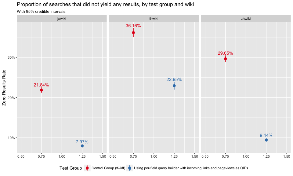
Figure 2: Zero results rate is the proportion of searches in which the user received zero results. Broken down by test group and wiki.
PaulScore
In Figure 3, we see that the test group had slightly lower PaulScores, which indicates that the results were less relevant. The difference is not significant when F = 0.9. This make sense because the smaller the value of scoring factor, the more weight put on the first few results, with lower ranking results counting for almost nothing. F=0.9 takes into account the broadest range of result rankings, and thus is less likely to change as dramatically. Figure 4 shows that zhwiki had the largest PaulScore differences between control and test group.
set.seed(777)
paulscores <- searches %>%
  ungroup %>%
  filter(clickthrough==TRUE) %>% #???
  select(c(`test group`, `Query score (F=0.1)`, `Query score (F=0.5)`, `Query score (F=0.9)`)) %>%
  gather(`F value`, `Query score`, -`test group`) %>%
  mutate(`F value` = sub("^Query score \\(F=(0\\.[159])\\)$", "F = \\1", `F value`)) %>%
  group_by(`test group`, `F value`) %>%
  summarize(
    PaulScore = mean(`Query score`),
    Interval = paste0(quantile(bootstrap_mean(`Query score`, 1000), c(0.025, 0.975)), collapse = ",")
  ) %>%
  extract(Interval, into = c("Lower", "Upper"), regex = "(.*),(.*)", convert = TRUE)
paulscores %>%
ggplot(aes(x = `F value`, y = PaulScore, color = `test group`)) +
geom_pointrange(aes(ymin = Lower, ymax = Upper), position = position_dodge(width = 0.7)) +
scale_color_brewer("Test Group", palette = "Set1", guide = guide_legend(ncol = 2)) +
#scale_y_continuous(limits = c(0.2, 0.35)) +
labs(x = NULL, y = "PaulScore(F)",
title = "PaulScore(F) by test group and value of F",
subtitle = "With bootstrapped 95% confidence intervals.") +
geom_text(aes(label = sprintf("%.3f", PaulScore), y = Upper + 0.01, vjust = "bottom"),
position = position_dodge(width = 0.7)) +
theme(legend.position = "bottom") 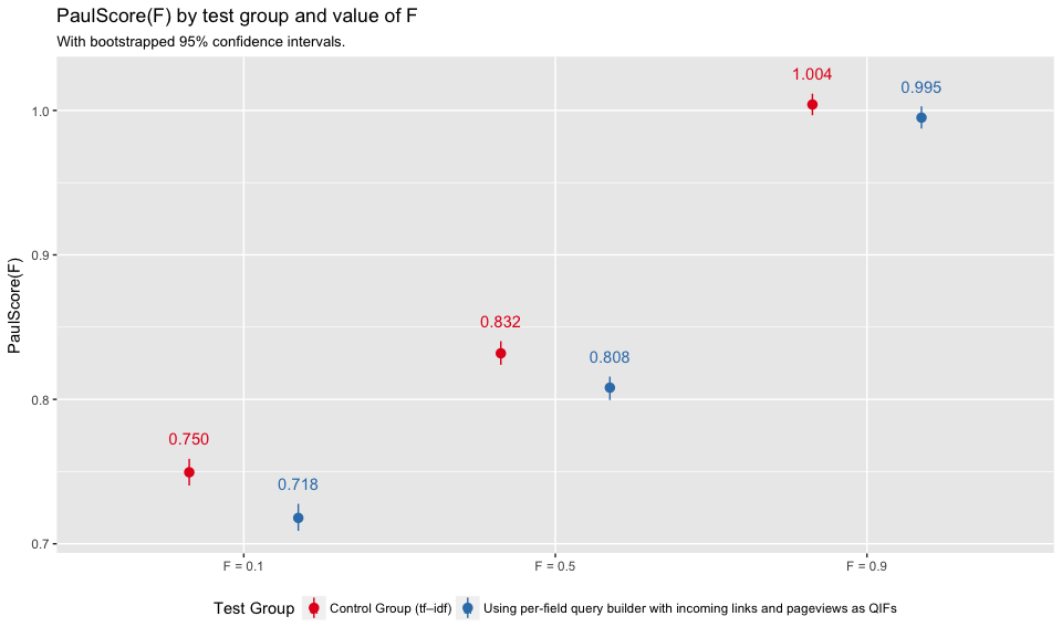
Figure 3: Average per-group PaulScore for various values of F (0.1, 0.5, and 0.9) with bootstrapped confidence intervals.
set.seed(777)
paulscores <- searches %>%
  ungroup %>%
  filter(clickthrough==TRUE) %>%
  select(c(wiki, `test group`, `Query score (F=0.1)`, `Query score (F=0.5)`, `Query score (F=0.9)`)) %>%
  gather(`F value`, `Query score`, -c(`test group`, wiki)) %>%
  mutate(`F value` = sub("^Query score \\(F=(0\\.[159])\\)$", "F = \\1", `F value`)) %>%
  group_by(wiki, `test group`, `F value`) %>%
  summarize(
    PaulScore = mean(`Query score`),
    Interval = paste0(quantile(bootstrap_mean(`Query score`, 1000), c(0.025, 0.975)), collapse = ",")
  ) %>%
  extract(Interval, into = c("Lower", "Upper"), regex = "(.*),(.*)", convert = TRUE)
paulscores %>%
  ggplot(aes(x = `F value`, y = PaulScore, color = `test group`)) +
  geom_pointrange(aes(ymin = Lower, ymax = Upper), position = position_dodge(width = 0.7)) +
  scale_color_brewer("Test Group", palette = "Set1", guide = guide_legend(ncol = 2)) +
  #scale_y_continuous(limits = c(0.2, 0.35)) +
  labs(x = NULL, y = "PaulScore(F)",
       title = "PaulScore(F) by wiki, test group and value of F",
       subtitle = "With bootstrapped 95% confidence intervals.") +
  geom_text(aes(label = sprintf("%.3f", PaulScore), y = Upper + 0.01, vjust = "bottom"),
            position = position_dodge(width = 0.7)) +
  facet_wrap(~ wiki, ncol = 3) +
theme(legend.position = "bottom") 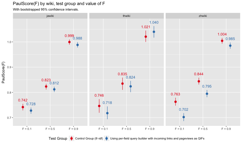
Figure 4: Average per-group PaulScore for various values of F (0.1, 0.5, and 0.9) with bootstrapped confidence intervals. Broken down by test group and wiki.
Engagement
In Figure 5, we see that the test group had a significantly lower clickthrough rate, which means users are less engaged with their search results. Again, zhwiki shows the largest discrepancy between control and test group in Figure 6.
engagement_overall <- searches %>%
  filter(results=="some") %>% #???
  group_by(`test group`) %>%
  summarize(clickthroughs = sum(clickthrough > 0),
            searches = n(), ctr = clickthroughs/searches) %>%
  ungroup
engagement_overall <- cbind(
  engagement_overall,
  as.data.frame(
    binom:::binom.bayes(
      engagement_overall$clickthroughs,
      n = engagement_overall$searches)[, c("mean", "lower", "upper")]
  )
)
engagement_overall %>%
ggplot(aes(x = 1, y = mean, color = `test group`)) +
geom_pointrange(aes(ymin = lower, ymax = upper), position = position_dodge(width = 1)) +
scale_color_brewer("Test Group", palette = "Set1", guide = guide_legend(ncol = 2)) +
scale_y_continuous(labels = scales::percent_format(), expand = c(0.01, 0.01)) +
labs(x = NULL, y = "Clickthrough rate",
title = "Engagement with search results by test group") +
geom_text(aes(label = sprintf("%.1f%%", 100 * ctr), y = upper + 0.0025, vjust = "bottom"),
position = position_dodge(width = 1)) +
theme(legend.position = "bottom")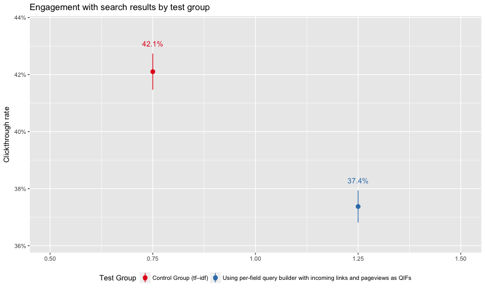
Figure 5: Clickthrough rates of test groups.
engagement_overall <- searches %>%
  filter(results=="some") %>%
  group_by(wiki, `test group`) %>%
  summarize(clickthroughs = sum(clickthrough > 0),
            searches = n(), ctr = clickthroughs/searches) %>%
  ungroup
engagement_overall <- cbind(
  engagement_overall,
  as.data.frame(
    binom:::binom.bayes(
      engagement_overall$clickthroughs,
      n = engagement_overall$searches)[, c("mean", "lower", "upper")]
  )
)
engagement_overall %>%
  ggplot(aes(x = 1, y = mean, color = `test group`)) +
  geom_pointrange(aes(ymin = lower, ymax = upper), position = position_dodge(width = 1)) +
  scale_color_brewer("Test Group", palette = "Set1", guide = guide_legend(ncol = 2)) +
  scale_y_continuous(labels = scales::percent_format(), expand = c(0.01, 0.01)) +
  labs(x = NULL, y = "Clickthrough rate",
       title = "Engagement with search results by test group and wiki") +
  geom_text(aes(label = sprintf("%.1f%%", 100 * ctr), y = upper + 0.0025, vjust = "bottom"),
            position = position_dodge(width = 1)) +
  facet_wrap(~ wiki, ncol = 3) +
  theme(legend.position = "bottom")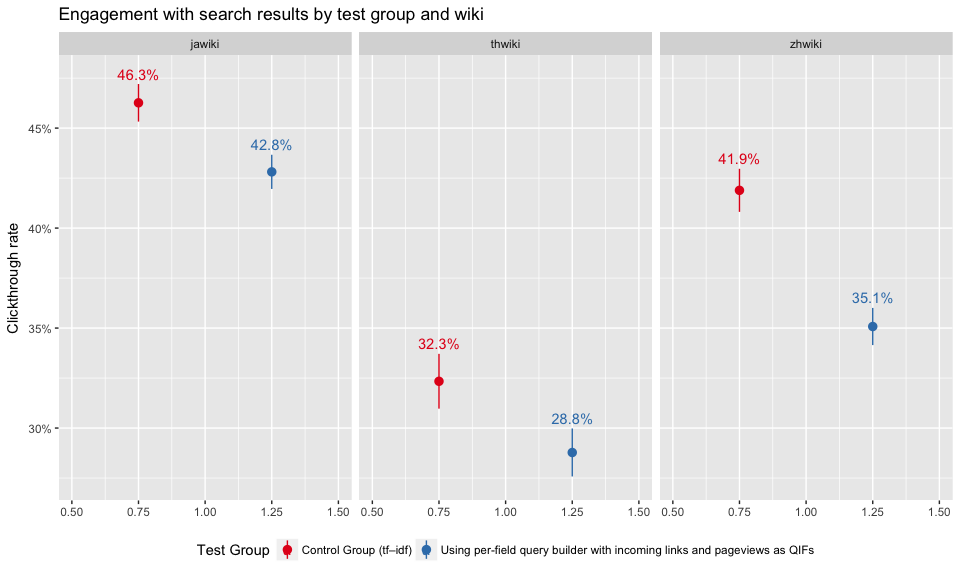
Figure 6: Clickthrough rates broken down by test group and wiki.
First Clicked Result’s Position
In Figure 7, we see that test group users were less likely to click on the first search result first than the control group. Figure 8 shows that only zhwiki users first clicked on the first result at a significantly lower rate, which indicates that the results were less relevant.
safe_ordinals <- function(x) {
  return(vapply(x, toOrdinal::toOrdinal, ""))
}
first_clicked <- searches %>%
  filter(results == "some" & clickthrough & !is.na(`first clicked result's position`)) %>%
  mutate(`first clicked result's position` = ifelse(`first clicked result's position` < 4, safe_ordinals(`first clicked result's position` + 1), "5th or higher")) %>%
  group_by(`test group`, `first clicked result's position`) %>%
  tally %>%
  mutate(total = sum(n), prop = n/total) %>%
  ungroup
set.seed(0)
temp <- as.data.frame(binom:::binom.bayes(first_clicked$n, n = first_clicked$total, tol = .Machine$double.eps^0.1)[, c("mean", "lower", "upper")])
first_clicked <- cbind(first_clicked, temp); rm(temp)
first_clicked %>%
ggplot(aes(x = 1, y = mean, color = `test group`)) +
geom_pointrange(aes(ymin = lower, ymax = upper), position = position_dodge(width = 1)) +
geom_text(aes(label = sprintf("%.1f", 100 * prop), y = upper + 0.0025, vjust = "bottom"),
position = position_dodge(width = 1)) +
scale_y_continuous(labels = scales::percent_format(),
expand = c(0, 0.005), breaks = seq(0, 1, 0.01)) +
scale_color_brewer("Test Group", palette = "Set1", guide = guide_legend(ncol = 2)) +
facet_wrap(~ `first clicked result's position`, scale = "free_y", nrow = 1) +
labs(x = NULL, y = "Proportion of searches",
title = "Position of the first clicked result",
subtitle = "With 95% credible intervals") +
theme(legend.position = "bottom",
panel.grid.major.x = element_blank(),
panel.grid.minor.x = element_blank(),
axis.ticks.x = element_blank(),
axis.text.x = element_blank(),
strip.background = element_rect(fill = "gray90"),
panel.border = element_rect(color = "gray30", fill = NA))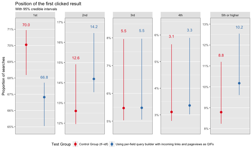
Figure 7: First clicked result’s position by test group.
first_clicked <- searches %>%
  filter(results == "some" & clickthrough & !is.na(`first clicked result's position`)) %>%
  mutate(`first clicked result's position` = ifelse(`first clicked result's position` < 4, safe_ordinals(`first clicked result's position` + 1), "5th or higher")) %>%
  group_by(wiki, `test group`, `first clicked result's position`) %>%
  tally %>%
  mutate(total = sum(n), prop = n/total) %>%
  ungroup
set.seed(0)
temp <- as.data.frame(binom:::binom.bayes(first_clicked$n, n = first_clicked$total, tol = .Machine$double.eps^0.1)[, c("mean", "lower", "upper")])
first_clicked <- cbind(first_clicked, temp); rm(temp)
first_clicked %>%
  ggplot(aes(x = 1, y = mean, color = `test group`)) +
  geom_pointrange(aes(ymin = lower, ymax = upper), position = position_dodge(width = 1)) +
  geom_text(aes(label = sprintf("%.1f", 100 * prop), y = upper + 0.0025, vjust = "bottom"),
            position = position_dodge(width = 1)) +
  scale_y_continuous(labels = scales::percent_format(),
                     expand = c(0, 0.005), breaks = seq(0, 1, 0.01)) +
  scale_color_brewer("Test Group", palette = "Set1", guide = guide_legend(ncol = 2)) +
  facet_wrap(~ wiki+`first clicked result's position`, scale = "free_y", ncol=5, nrow = 3) +
  labs(x = NULL, y = "Proportion of searches",
       title = "Position of the first clicked result",
       subtitle = "With 95% credible intervals") +
  theme(legend.position = "bottom",
        panel.grid.major.x = element_blank(),
        panel.grid.minor.x = element_blank(),
        axis.ticks.x = element_blank(),
        axis.text.x = element_blank(),
        strip.background = element_rect(fill = "gray90"),
        panel.border = element_rect(color = "gray30", fill = NA))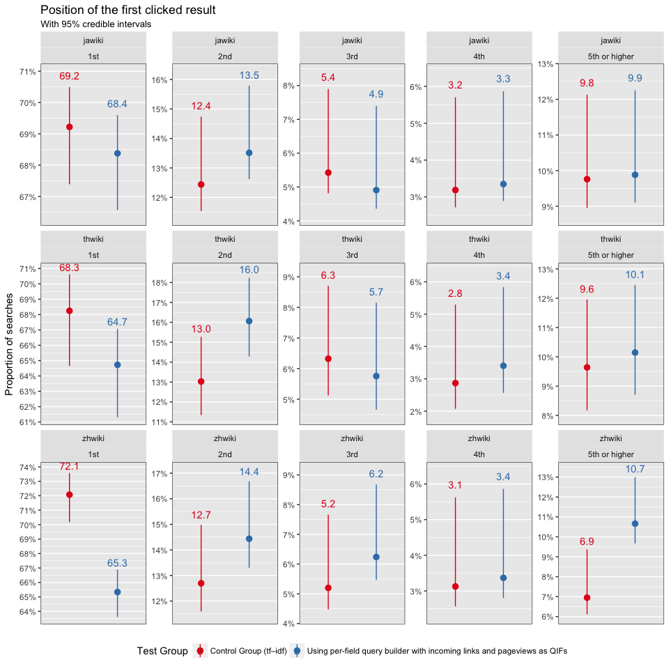
Figure 8: First clicked result’s position by test group and wiki.
Dwell Time per Visited Page
Figures 9 and 10 show the survival curve for each test group and wiki. Except zhwiki, users are more likely to stay longer on visited pages, which implies the results in test group are more relevant for jawiki and thwiki.
clickedResults %>%
  split(.$`test group`) %>%
  map_df(function(df) {
    seconds <- c(0, 10, 20, 30, 40, 50, 60, 90, 120, 150, 180, 210, 240, 300, 360, 420)
    seshs <- as.data.frame(do.call(cbind, lapply(seconds, function(second) {
      return(sum(df$dwell_time >= second))
    })))
    names(seshs) <- seconds
    return(cbind(`test group` = head(df$`test group`, 1), n = seshs$`0`, seshs, `450`=seshs$`420`))
  }) %>%
  gather(seconds, visits, -c(`test group`, n)) %>%
  mutate(seconds = as.numeric(seconds)) %>%
  group_by(`test group`, seconds) %>%
  mutate(proportion = visits/n) %>%
  ungroup() %>%
  ggplot(aes(group=`test group`, color=`test group`)) +
  geom_step(aes(x = seconds, y = proportion), direction = "hv") +
  scale_x_continuous(name = "T (Dwell Time in seconds)", breaks=c(0, 10, 20, 30, 40, 50, 60, 90, 120, 150, 180, 210, 240, 300, 360, 420))+
  scale_y_continuous("Proportion of visits longer than T (P%)", labels = scales::percent_format(),
                     breaks = seq(0, 1, 0.1)) +
  scale_color_brewer(palette = "Set1") +
  theme(legend.position = "bottom")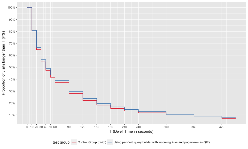
Figure 9: At time T, at most P% of users still stay on their visited pages. Broken down by test group.
clickedResults %>%
  split(list(.$wiki, .$`test group`)) %>%
  map_df(function(df) {
    seconds <- c(0, 10, 20, 30, 40, 50, 60, 90, 120, 150, 180, 210, 240, 300, 360, 420)
    seshs <- as.data.frame(do.call(cbind, lapply(seconds, function(second) {
      return(sum(df$dwell_time >= second))
    })))
    names(seshs) <- seconds
    return(cbind(wiki=head(df$wiki, 1), `test group` = head(df$`test group`, 1), n = seshs$`0`, seshs, `450`=seshs$`420`))
  }) %>%
  gather(seconds, visits, -c(wiki, `test group`, n)) %>%
  mutate(seconds = as.numeric(seconds)) %>%
  group_by(wiki, `test group`, seconds) %>%
  mutate(proportion = visits/n) %>%
  ungroup() %>%
  ggplot(aes(group=`test group`, color=`test group`)) +
  geom_step(aes(x = seconds, y = proportion), direction = "hv") +
  scale_x_continuous(name = "T (Dwell Time in seconds)", breaks=c(0, 10, 20, 30, 40, 50, 60, 90, 120, 150, 180, 210, 240, 300, 360, 420))+
  scale_y_continuous("Proportion of visits longer than T (P%)", labels = scales::percent_format(),
                     breaks = seq(0, 1, 0.1)) +
  scale_color_brewer(palette = "Set1") +
  theme(legend.position = "bottom") +
  facet_wrap(~ wiki, ncol=1, nrow =3)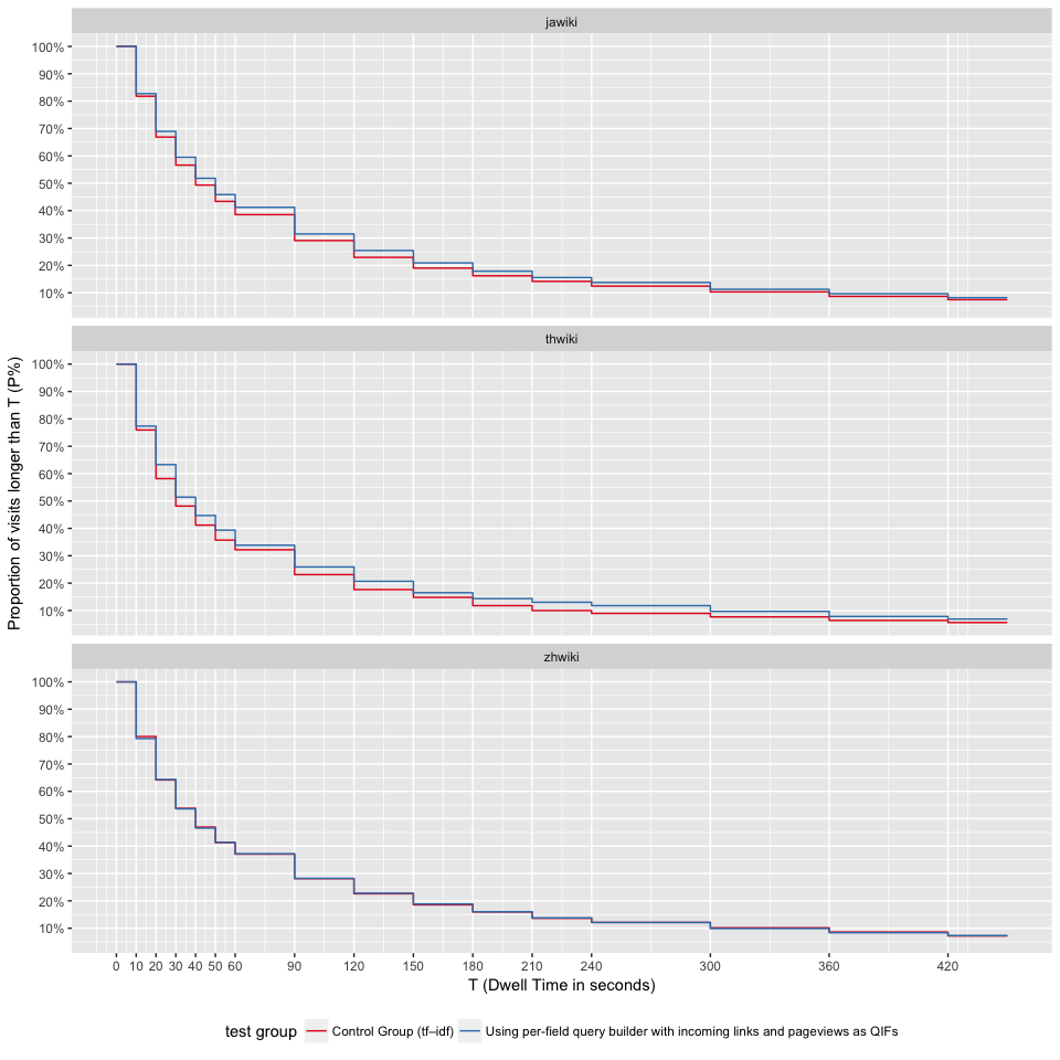
Figure 10: At time T, at most P% of users still stay on their visited pages. Broken down by test group and wiki.
Scroll
In Figures 11 and 12, we can see that users in the test group are more likely to scroll on the visited pages, but the differences are not statistically significant.
scroll_overall <- clickedResults %>%
  group_by(`test group`) %>%
  summarize(scrolls=sum(scroll), visits=n(), proportion = sum(scroll)/n()) %>%
  ungroup
scroll_overall <- cbind(
  scroll_overall,
  as.data.frame(
    binom:::binom.bayes(
      scroll_overall$scrolls,
      n = scroll_overall$visits)[, c("mean", "lower", "upper")]
  )
)
scroll_overall %>%
  ggplot(aes(x = 1, y = mean, color = `test group`)) +
  geom_pointrange(aes(ymin = lower, ymax = upper), position = position_dodge(width = 1)) +
  scale_color_brewer("Test Group", palette = "Set1", guide = guide_legend(ncol = 2)) +
  scale_y_continuous(labels = scales::percent_format(), expand = c(0.01, 0.01)) +
  labs(x = NULL, y = "Proportion of visits",
       title = "Proportion of visits with scroll by test group") +
  geom_text(aes(label = sprintf("%.1f%%", 100 * proportion), y = upper + 0.0025, vjust = "bottom"),
            position = position_dodge(width = 1)) +
  theme(legend.position = "bottom")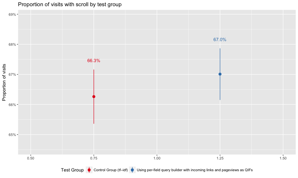
Figure 11: Proportion of visited pages with scroll by test group.
scroll_overall <- clickedResults %>%
  group_by(wiki, `test group`) %>%
  summarize(scrolls=sum(scroll), visits=n(), proportion = sum(scroll)/n()) %>%
  ungroup
scroll_overall <- cbind(
  scroll_overall,
  as.data.frame(
    binom:::binom.bayes(
      scroll_overall$scrolls,
      n = scroll_overall$visits)[, c("mean", "lower", "upper")]
  )
)
scroll_overall %>%
  ggplot(aes(x = 1, y = mean, color = `test group`)) +
  geom_pointrange(aes(ymin = lower, ymax = upper), position = position_dodge(width = 1)) +
  scale_color_brewer("Test Group", palette = "Set1", guide = guide_legend(ncol = 2)) +
  scale_y_continuous(labels = scales::percent_format(), expand = c(0.01, 0.01)) +
  labs(x = NULL, y = "Proportion of visits",
       title = "Proportion of visits with scroll by test group and wiki") +
  geom_text(aes(label = sprintf("%.1f%%", 100 * proportion), y = upper + 0.0025, vjust = "bottom"),
            position = position_dodge(width = 1)) +
  facet_wrap(~ wiki, ncol = 3) +
  theme(legend.position = "bottom")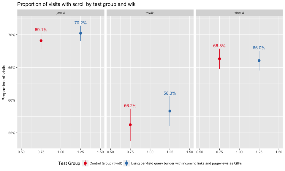
Figure 12: Proportion of visited pages with scroll by test group and wiki.
Query Reformulation
First, we tokenized queries from zhwiki, jawiki and thwiki with jieba, tinysegmenter and elasticsearch termvectors api separately. Then we filter out stop words.
# See tokenize.R for more details
library(jiebaR)
library(ropencc)

#thwiki
load("../data/tokens_th.RData")
tokens_th <- output; rm(output)
stopword_th <- jsonlite::fromJSON("../resource/th.json")
tokens_th <- filter_segment(tokens_th,stopword_th)

#zhwiki
queries_zh <- searches[searches$wiki=="zhwiki", c("page_id","query")]
queries_zh$query <- gsub("[[:punct:]]", " ", queries_zh$query)
stopword_zh <- jsonlite::fromJSON("../resource/zh.json")
ccst = converter(S2T)
stopword_zh <- union(ccst[stopword_zh], stopword_zh)
mixseg = worker(bylines = TRUE)
tokens_zh <- mixseg[queries_zh$query]
tokens_zh <- filter_segment(tokens_zh,stopword_zh)
names(tokens_zh) <- queries_zh$page_id

#jawiki
tokens_ja <- jsonlite::fromJSON("../data/tokens_ja.json")
stopword_ja <- jsonlite::fromJSON("../resource/ja.json")
tokens_ja <- filter_segment(tokens_ja,stopword_ja)
tokens_ja <- lapply(tokens_ja, function(x) gsub(" +","",x)) # strip space before/after string
We consider two queries as a reformulation if 1) they are from the same search session and share at least one result, or 2) they are from the same search session and share at least one word.
library(igraph)
all_tokens <- c(tokens_ja, tokens_zh, tokens_th)

overlapping_results <- function(x) {
  if (all(is.na(x))) {
    return(diag(length(x)))
  }
  input <- strsplit(stringr::str_replace_all(x, "[\\[\\]]", ""), ",")
  output <- vapply(input, function(y) {
    temp <- vapply(input, function(z) { length(intersect(z, y)) }, 0L)
    temp[is.na(x)] <- 0L
    return(temp)
  }, rep(0L, length(input)))
  diag(output) <- 1L
  return(output)
}

reformulation <- function(result_pids, page_ids, all_tokens) {
  if(length(page_ids)==1){
    return(data.frame(n_search=1, n_reformulate="0"))
  }
  # result overlap
  overlaps_res <- overlapping_results(result_pids)
  # tokens overlap
  this_tokens <- all_tokens[page_ids]
  overlaps_token <- vapply(this_tokens, function(y) {
    temp <- vapply(this_tokens, function(z) { length(intersect(z, y)) }, 0L)
    temp[is.na(this_tokens)] <- 0L
    return(temp)
  }, rep(0L, length(this_tokens)))
  diag(overlaps_token) <- 1L

  overlaps_all <- (overlaps_res + overlaps_token) > 0
  diag(overlaps_all) <- 0L
  graph_object <- graph_from_adjacency_matrix(overlaps_all, mode = c("undirected"), diag = F)
  csize <- clusters(graph_object)$csize
  return(data.frame(n_search=length(csize), n_reformulate=ifelse(length(csize)>1,paste(csize-1, collapse=',' ), as.character(csize-1))))
}

reform_times <- searches %>%
  group_by(wiki, `test group`, session_id, search_id) %>%
  do(reformulation(.$`result page IDs`, .$page_id, all_tokens))
We grouped connected searches together using the rules above, then we have 51354 total search groups.
reform_times %>% ungroup %>%
  mutate(n_search=ifelse(n_search>=10,"10+",n_search)) %>%
  group_by(n_search) %>%
  summarise(n_session=n()) %>%
  mutate(prop=n_session/sum(n_session)) %>%
  ggplot(aes(x = n_search, y = prop)) +
  geom_bar(stat = "identity") +
  scale_y_continuous("Proportion of search sessions", labels = scales::percent_format()) +
  scale_x_discrete("Number of Search Groups", limits = c(1:9, "10+")) +
  geom_text(aes(label = sprintf("%.1f%%", 100*prop)), nudge_y = 0.025) +
  ggthemes::theme_tufte(base_family = "Gill Sans", base_size = 14) +
  ggtitle("Proportion of search sessions making N search groups")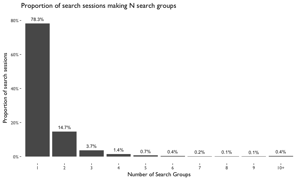
Figure 13: Proportion of search sessions making N search groups. A search group is a group of searches from the same search session, in which one search is connected with at least another one if they share at least one common word or at least one common result.
In Figure 14 and Figure 16, we can see that test group users are less likely to reformulate their queries. Figure 15 and Figure 17 show that zhwiki had the largest discrepancy between control and test group.
reformulation_counts <- reform_times %>%
  group_by(`test group`) %>%
  summarize(`searches with query reformulations` = sum(as.numeric(unlist(lapply(n_reformulate, function(x) strsplit(x, ",")))) > 0),
            searches = sum(n_search),
            proportion = `searches with query reformulations`/searches) %>%
  ungroup
reformulation_counts <- cbind(
  reformulation_counts,
  as.data.frame(
    binom:::binom.bayes(
      reformulation_counts$`searches with query reformulations`,
      n = reformulation_counts$searches,
      tol = .Machine$double.eps^0.1)[, c("mean", "lower", "upper")]
  )
)
reformulation_counts %>%
  ggplot(aes(x = `test group`, y = `mean`, color = `test group`)) +
  geom_pointrange(aes(ymin = lower, ymax = upper)) +
  scale_x_discrete(limits = levels(events$test_group)) +
  scale_y_continuous(labels = scales::percent_format()) +
  scale_color_brewer("Test Group", palette = "Set1", guide = FALSE) +
  labs(x = NULL, y = "% of searches with query reformulations",
       title = "Searches with reformulated queries by test group",
       subtitle = "Queries were grouped when they shared common results or common key words") +
  geom_text(aes(label = sprintf("%.2f%%", 100 * proportion),
                vjust = "bottom", hjust = "center"), nudge_x = 0.1)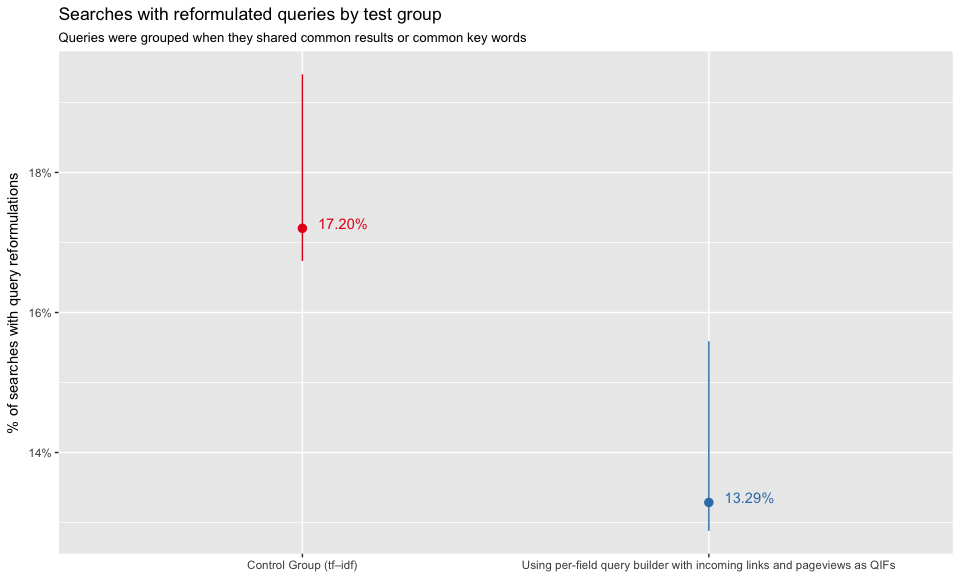
Figure 14: Proportions of searches where user reformulated their query.
reformulation_counts <- reform_times %>%
  group_by(wiki, `test group`) %>%
  summarize(`searches with query reformulations` = sum(as.numeric(unlist(lapply(n_reformulate, function(x) strsplit(x, ",")))) > 0),
            searches = sum(n_search),
            proportion = `searches with query reformulations`/searches) %>%
  ungroup
reformulation_counts <- cbind(
  reformulation_counts,
  as.data.frame(
    binom:::binom.bayes(
      reformulation_counts$`searches with query reformulations`,
      n = reformulation_counts$searches)[, c("mean", "lower", "upper")]
  )
)
reformulation_counts %>%
  ggplot(aes(x = 1, y = `mean`, color = `test group`)) +
  geom_pointrange(aes(ymin = lower, ymax = upper), position = position_dodge(width = 1)) +
  scale_y_continuous(labels = scales::percent_format(), expand = c(0.01, 0.01)) +
  scale_color_brewer("Test Group", palette = "Set1", guide = guide_legend(ncol = 2)) +
  labs(x = NULL, y = "% of searches with query reformulations",
       title = "Searches with reformulated queries by test group and wiki",
       subtitle = "Queries were grouped when they shared common results or common key words") +
  geom_text(aes(label = sprintf("%.1f%%", 100 * proportion), y = upper + 0.0025, vjust = "bottom"),
            position = position_dodge(width = 1)) +
  theme(legend.position = "bottom")+
  facet_wrap(~ wiki, ncol = 3)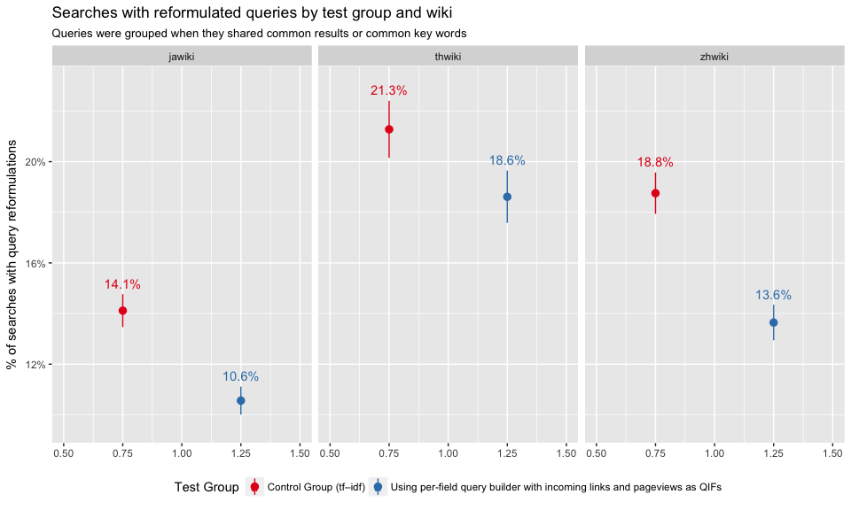
Figure 15: Proportions of searches where user reformulated their query. Broken down by wiki.
count_reformulation <- function(n_reformulate){
  temp <- as.numeric(unlist(lapply(n_reformulate, function(x) strsplit(x, ","))))
  temp <- ifelse(temp>=3, "3+", temp)
  output <- as.data.frame(table(temp))
  output$proportion <- output$Freq/sum(output$Freq)
  colnames(output)[1] <- "query reformulations"
  return(output)
}
reform_times %>%
  group_by(`test group`) %>%
  do(count_reformulation(.$n_reformulate)) %>%
  ggplot(aes(x = `query reformulations`, y = proportion, fill = `test group`)) +
  geom_bar(stat = "identity", position = "dodge") +
  scale_y_continuous(labels = scales::percent_format()) +
  scale_fill_brewer("Test Group", palette = "Set1", guide = guide_legend(ncol = 2)) +
  geom_text(aes(label = sprintf("%.1f%%", 100 * proportion), vjust = -0.5),
            position = position_dodge(width = 1)) +
  labs(y = "Proportion of searches", x = "Approximate number of query reformulations per grouped search",
       title = "Number of query reformulations by test group",
       subtitle = "Queries were grouped when they shared common results or common key words") +
  theme(legend.position = "bottom")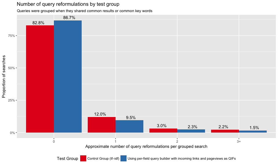
Figure 16: Proportions of searches with 0, 1, 2, and 3+ query reformulations.
reform_times %>%
  group_by(wiki, `test group`) %>%
  do(count_reformulation(.$n_reformulate)) %>%
  ggplot(aes(x = `query reformulations`, y = proportion, fill = `test group`)) +
  geom_bar(stat = "identity", position = "dodge") +
  scale_y_continuous(labels = scales::percent_format()) +
  scale_fill_brewer("Test Group", palette = "Set1", guide = guide_legend(ncol = 2)) +
  geom_text(aes(label = sprintf("%.1f%%", 100 * proportion), vjust = -0.5),
            position = position_dodge(width = 1)) +
  labs(y = "Proportion of searches", x = "Approximate number of query reformulations per grouped search",
       title = "Number of query reformulations by test group and wiki",
       subtitle = "Queries were grouped when they shared common results or common key words") +
  theme(legend.position = "bottom")+
  facet_wrap(~ wiki, ncol = 3)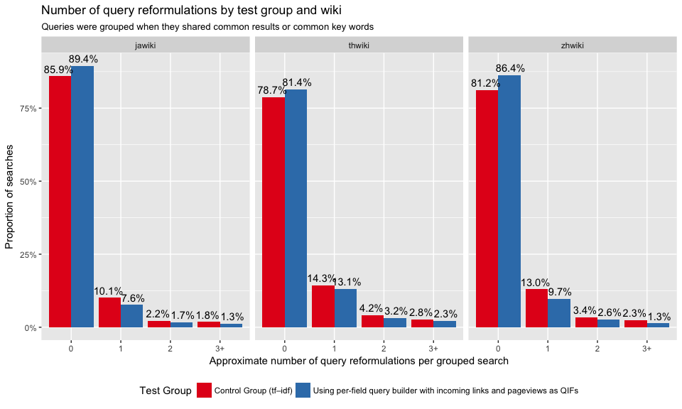
Figure 17: Proportions of searches with 0, 1, 2, and 3+ query reformulations. Broken down by wiki.
Conclusion and Discussion
For the test group, we observed a much better ZRR but slightly worse PaulScores, large decrease in clickthrough rate, and fewer users clicked on the first result first, indicating that we are showing users worse results. However, dwell-time and query reformulation analysis show that users may like the results they are getting in some aspect. We recommend deploying BM25 for all wikis but not reindexing projects in space-less languages for now.
This test revealed the performance of BM25 is unsatisfactory on space-less languages: some CirrusSearch components are dependent on the presence of spaces. We agree that the current behavior (forcing a proximity match on every query) is far from ideal but given the outcome of the test we decided not to move forward without prior work on space-less languages. We need better tokenization, and we need to track and fix all the components that make the bold assumption of the presence of spaces to activate/deactivate features.
The relatively large decrease in engagement and relevancy for zhwiki may be the result of tokenizer behavior. Chinese is the sole language in this test where we do not have a custom analysis chain. We emit only unigrams, so any page that randomly has all the same characters as the query in it will be returned. This can greatly decreases ZRR without any increase in search result quality or relevance. In English this would be roughly similar to returning any page that had all the same letters as the query.
The query reformulation analysis in this report is not ideal. Firstly, finding out shared tokens could not detect reformulated queries when users fix a typo in space-less languages. For example, when users modify their queries from “灯龙” to “灯笼” (lantern) they are fixing a typo, but tokenizers would take them as two different words. Secondly, we found that many users like to try their queries in different languages. Without enabling search across wikis in different languages, we are unable to detect this kind of reformulation.