Search Relevance Surveys and Deep Learning
Turning Noisy, Crowd-sourced Opinions Into An Accurate Relevance Judgement
Erik Bernhardson
Trey Jones
Mikhail Popov
Deb Tankersley
01 December 2017
Abstract
To improve the relevance of search results on Wikipedia and other Wikimedia Foundation projects, the Search Platform team has focused endeavor on ranking results with machine learning. The first iteration used a click-based model to create relevance labels. Here we present a way to augment that training data with a deep neural network (although other models are also considered) that can predict relevance of a wiki page to a specific search query based on users’ responses to the question “If someone searched for ‘…’, would they want to read this article?”. The model has 80% overall accuracy but over 90% accuracy when there are at least 40 responses and 100% accuracy when there are 70 or more responses. Once deployed, we can utilize users’ responses to search relevance surveys and this model to create relevance labels for training the ranker.
![]() Phabricator ticket |
Phabricator ticket | ![]() Open source analysis |
Open source analysis | ![]() Open data
Open data
Introduction
Our current efforts to improve relevance of search results on Wikipedia and other Wikimedia Foundation projects are focused on information retrieval using machine-learned ranking (MLR). In MLR, a model is trained to predict a document’s relevance from various document-level and query-level features which represent the document. The first iteration used a click-based Dynamic Bayesian Network (implemented via ClickModels Python library) to create relevance labels for training data fed into XGBoost. For further details, please refer to First assessment of learning-to-rank: testing machine-learned ranking of search results on English Wikipedia.
To augment the click-based training data that the ranking model uses, we decided to try crowd-sourcing relevance opinions. Our initial prototype showed promise, so we decided to up the scale. It was not feasible for us to manually grade thousands of pages to craft the golden standard, so instead we used a previously collected dataset of relevance scores from an earlier endeavor called Discernatron.
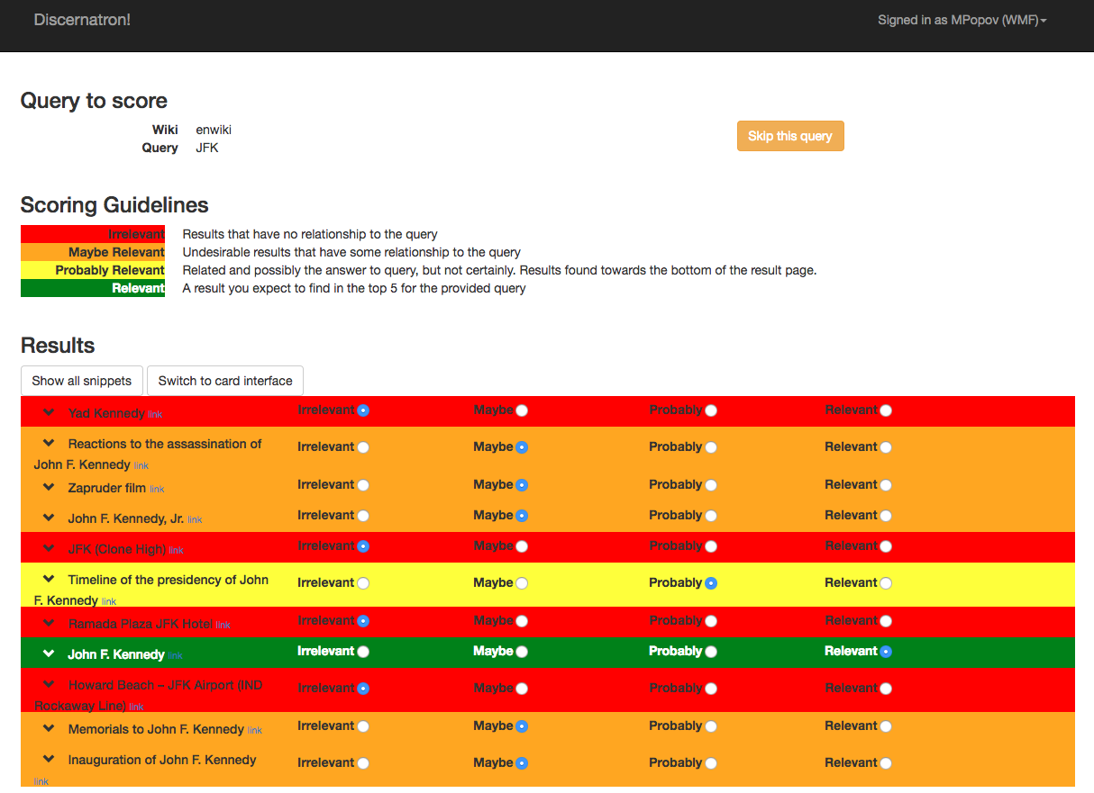
Discernatron is a search relevance tool developed by the Search Platform team (formerly Discovery department). Its goal was to help improve search relevance - showing articles that are most relevant to search queries - with human assistance. We asked for people to use Discernatron to review search suggestions across multiple search tools and respondents were presented with a set of search results from four tools - CirrusSearch (Wiki search), Bing, Google, and DuckDuckGo. For each query, users were provided with the set of titles found and asked to rank each title from 1 to 4, or leave the title unranked. For each query - result pair, we calculated an average score. After examining the scores, we decided that a score 0-1 indicated the result was “irrelevant” and a score greater than 1 (up to a maximum of 3) indicated the result was “relevant”. These are the labels we trained our model to predict.
However, since graders have different opinions and some scores are calculated from more data than others, we separated the scores into those which are “reliable” and those which are “unreliable” based on whether the Krippendorff’s alpha exceeded a threshold of 0.45. (Refer to RelevanceScoring/Reliability.php and RelevanceScoring/KrippendorffAlpha.php in Discernatron’s source code for implementation details.)
Methods
The (binary) classifiers trained are:
- logistic regression, generically coded as “multinom” in the Results tables
- shallow neural network (with 1 hidden layer), coded as “nnet” in the Results tables
- deep neural network with (with up to 3 hidden layers), coded as “dnn” in the Results tables
- naïve Bayes, coded as “nb” in the Results tables
- random forest, coded as “rf” in the Results tables
- gradient-boosted trees (via XGBoost), coded as “xgbTree” in the Results tables
- C5.0 trees, coded as “C5.0” in the Results tables
In addition to the 7 classifiers listed above (which we will refer to as base learners), we also trained a super learner in a technique called stacking. The base learners are trained in the first stage and are then asked to make predictions. Those predictions are then used as features (one feature for each base learner) to train the super learner in the second stage. Specifically, we chose Bayesian network (via the bnclassify package) as the super learner, coded as “meta” in the Results tables.
Furthermore, we trained a pair of deeper neural networks for binary classification. We utilized Keras with a TensorFlow backend and performed the training separately from the others, which is why they are not included as base learners in the stacked training of a super learner. The results from these two models are coded as “keras-1” and “keras-2” in the Results tables and they are specified as follows:
- keras-1: 3 hidden layers with 256, 128, and 64 units and dropout of 50%, 20%, and 10%, respectively.
- keras-2: 5 hidden layers with 128, 256, 128, 64, and 16 units and dropout of 50%, 50%, 50%, 25%, and 0%, respectively.
We utilized the caret package to perform hyperparameter tuning (via 5-fold cross-validation) and training (using 80% of the available data) of each base learner for a combination of each of the following:
- 4 questions we asked:
- “If someone searched for ‘…’, would they want to read this article?”
- “If you searched for ‘…’, would this article be a good result?”
- “If you searched for ‘…’, would this article be relevant?”
- “Would you click on this page when searching for ‘…’?”
- 2 types of Discernatron scores that would be discretized into labels: reliable vs unreliable
- 14 different feature sets:
- survey-only
- score summarizing users’ responses
- proportion who answered unsure
- engagement with the relevance survey
- survey & page info
- score, % unsure, engagement
- page size label based on page byte length:
- “tiny” (≤1 kB)
- “small” (1-10 kB)
- “medium” (10-50 kB)
- “large” (50-100 kB)
- “huge” (≥100 kB)
- indicator variables of whether the page is a:
- Category page
- Talk page
- File page
- list (e.g. “List of…”-type articles)
- survey & pageviews
- score, % unsure, engagement
- median pageview (pv) traffic during September 2017, categorized as:
- “no” (≤1 pvs/day)
- “low” (1-10 pvs/day)
- “medium” (10-100 pvs/day)
- “high” (100-1000 pvs/day)
- “very high” (≥1000 pvs/day)
- survey, page info, and traffic
- score, % unsure, engagement
- discrete page size and page type
- survey, page info, and traffic-by-weekday
- score, % unsure, engagement
- discrete page size and page type
- traffic on Monday-Sunday
- survey, page info, and traffic-by-platform
- score, % unsure, engagement
- discrete page size and page type
- traffic on desktop vs mobile web vs mobile app
- survey, page info, traffic-by-weekday, and traffic-by-platform
- score, % unsure, engagement
- discrete page size and page type
- traffic on Monday-Sunday
- traffic on desktop vs mobile web vs mobile app
- survey, page info, and traffic-by-platform-and-weekday
- score, % unsure, engagement
- discrete page size and page type
- traffic on weekday from platform (7x3=21 combinations)
- 6 configurations of survey, page info, page size, and pageviews
- score, % unsure, engagement, page type
- page size (in bytes) and pageviews (median/average in September 2017) using one of the following:
- raw values
- standardized (Z-score) raw values
- normalized raw values
- log10-transformed values
- standardized (Z-score) log10-transformed values
- normalized log10-transformed values
- survey-only
Standardization via means the predictor was centered around the mean and scaled by the standard deviation. Normalization was achieved via dividing by the maximum observed value and then subtracting 0.5 to center it around 0.
To correct for class imbalance – there were more irrelevant articles than relevant ones – instances were upsampled. In the case of Keras-constructed DNNs, we specified class weights such that the model paid slightly more attention to the less-represented “relevant” articles.
Results
Marginal accuracies
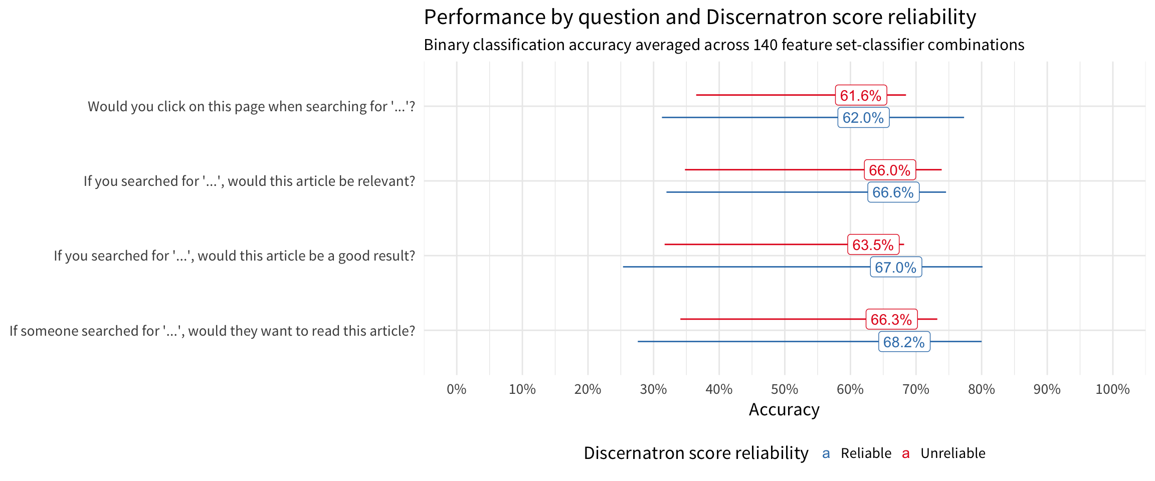
Models trained on reliable Discernatron scores have higher accuracy than models trained on unreliable Discernatron scores. The neutral question of “If someone…” worked better than the other questions which were aimed at the user.
| Classifier | Reliable Discernatron score | Unreliable Discernatron score |
|---|---|---|
| Logistic Regression (multinom) | 65.1% | 65.9% |
| Shallow NN (nnet) | 64.5% | 64.0% |
| Deep NN (dnn) | 67.5% | 66.0% |
| Deeper NN (keras-1) | 73.7% | 62.5% |
| Much Deeper NN (keras-2) | 63.0% | 58.4% |
| Naive Bayes (nb) | 53.7% | 40.0% |
| Random Forest (rf) | 66.5% | 65.1% |
| Gradient-boosted Trees (xgbTree) | 66.3% | 64.1% |
| C5.0 trees | 66.2% | 64.6% |
| Bayesian Network super learner (meta) | 62.0% | 61.4% |
Meta analysis
In this section, we fit a beta regression model of classification performance to the different components to help us see the impact of each component. We chose beta regression because accuracy is a value between 0 and 1, and this family of models enables us to work with that without transforming the response variable.
| component | estimate |
|---|---|
| (Intercept) | -0.0564 |
| reliability | 0.1602 |
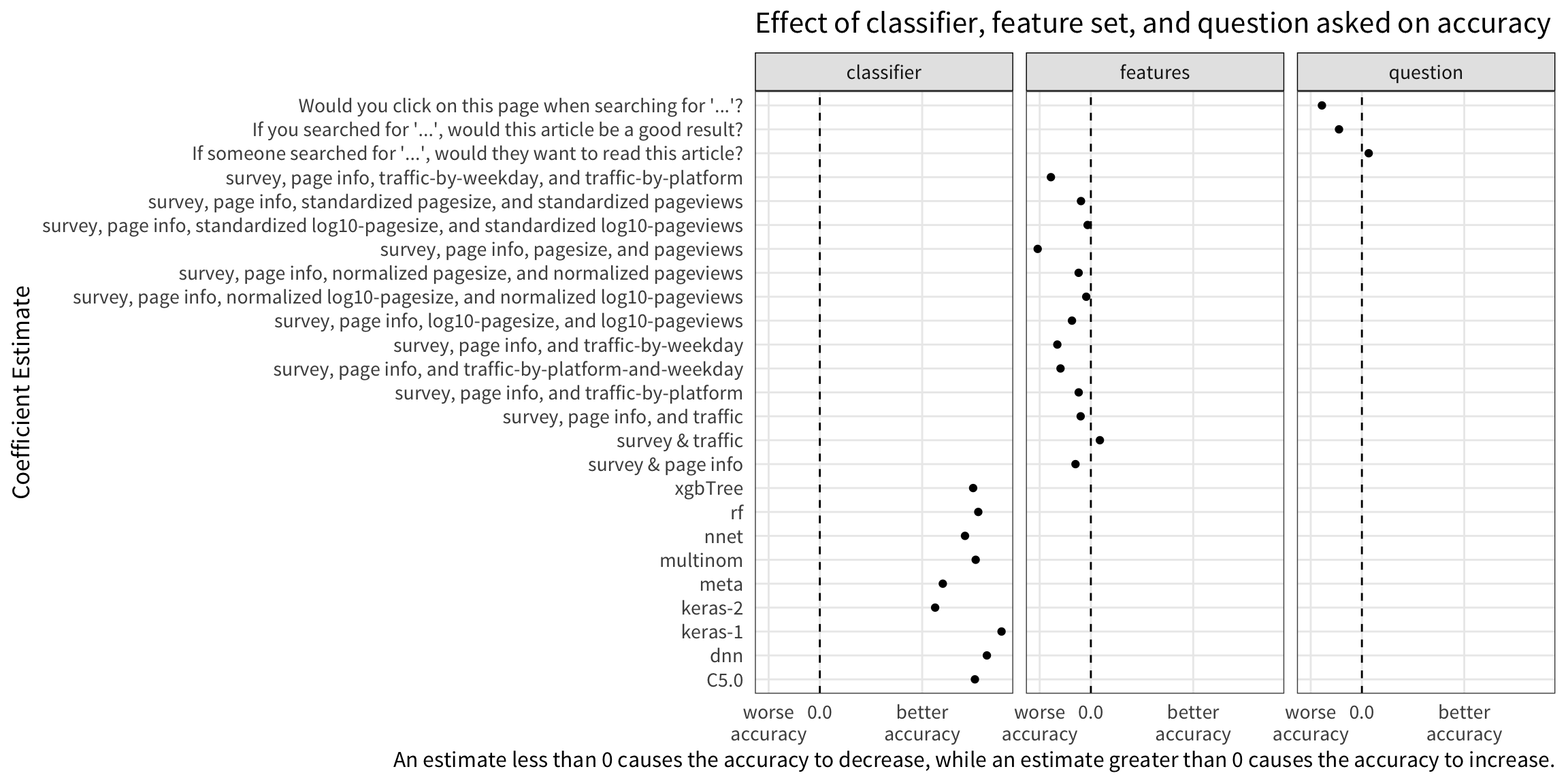
The baseline (intercept) is Naive Bayes classifier trained solely on responses to the question “If you searched for ‘…’, would this article be relevant?” Coefficient estimates for the intercept and reliability (shown in the table above) have been omitted from the figure for clarity.
After looking at the results of the beta regression in the table and figure, we came to the following conclusions:
- We should use reliable Discernatron scores, as that improved accuracy.
- Asking the neutrally phrased question “If someone searched for ‘…’, would they want to read this article?” lead to much better accuracy than the other questions which were directed at the user (“Would you…”, “If you searched…”).
- Using the deep neural network “keras-1” improved accuracy more than using other classifiers.
- Compared to just using survey responses, incorporating traffic data (in the form of categories such as “high”, “medium”, and “low”) slightly improved accuracy on average.
- Including page info (e.g. an indicator of whether it’s a Category or Talk page and the page size) did not help on average.
- Including pageview traffic (transformed, normalized, or otherwise) with page info had no impact on accuracy.
Responses required
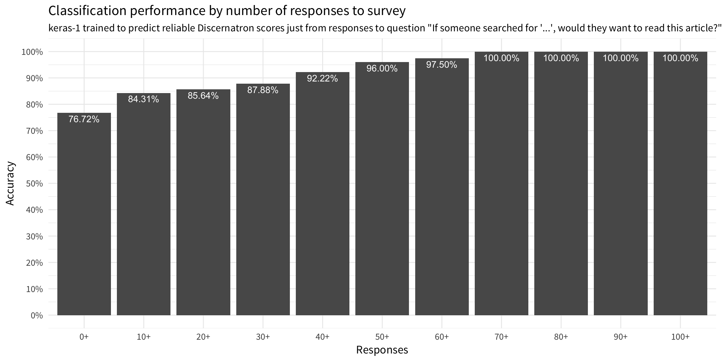
Relationship between number of survey responses to relevance prediction accuracy of keras-1 trained to predict reliable Discernatron scores just from responses to question “If someone searched for ‘…’, would they want to read this article?”
The model’s performance increases as we collect more responses to calculate the score from – the model is very accurate with at least 40 yes/no/unsure/dismiss responses and the most accurate with at least 70 responses. That is, we do not necessarily need to wait until we obtain at least 70 responses from users before we request a relevance prediction from the model, but we should wait until we have at least 40.
Accuracies by question
Question 1
Reliable Scores
Unreliable Scores
Question 2
Reliable Scores
Unreliable Scores
Question 3
Reliable Scores
Unreliable Scores
Question 4
Reliable Scores
Unreliable Scores
Conclusion & Discussion
By deploying “keras-1” trained just on survey responses to “If someone searched for…”, we will be able to classify a wiki page as relevant or irrelevant to a specific search query. In order to use the model to augment the training data for the ranking model, we should wait until we have at least 40 responses, but preferably until we have at least 70. Once we have sufficient number of responses, we can request a probability of relevance and then map that to a 0-10 scale that the ranking model expects.
The model can also be easily included in the pipeline for MjoLniR – our Python and Spark-based library for handling the backend data processing for Machine Learned Ranking at Wikimedia – because the final model was created with the Python-based Keras. Furthermore, since the final model uses only the survey response data and does not include additional data such as traffic or information about the page, the pipeline simply needs to calculate a score from users’ yes/no responses, the proportion of users who were unsure, and users’ engagement (responses/impressions) with the survey.
Finally, it would be interesting to evaluate how robust the models are to predicting relevance using response data from questions other than the one the model was trained with. For example, how well does the model trained on responses to “If someone searched for…” perform when it’s given responses to “If you searched for…”?
References & Software
- R Core Team (2017). R: A language and environment for statistical computing. R Foundation for Statistical Computing, Vienna, Austria. Software available from https://r-project.org
- Abadi, M. and others (2015). TensorFlow: Large-scale machine learning on heterogeneous systems. Software available from https://tensorflow.org
- Allaire, J.J. and Yuan Tang, Y. (2017). tensorflow: R Interface to ‘TensorFlow’. R package available from https://tensorflow.rstudio.com
- Chollet, F. and others (2015). Keras. Software available from https://keras.io
- Allaire, J.J. and Chollet, F. (2017). keras: R Interface to ‘Keras’. R package available from https://keras.rstudio.com
- Kuhn, M. (2017). caret: Classification and Regression Training. R package available from https://cran.r-project.org/package=caret
- Cribari-Neto, F. and Zeileis, A. (2010). Beta Regression in R. Journal of Statistical Software 34(2), 1-24. URL: https://www.jstatsoft.org/v34/i02/.
- Meyer, M., Dimitriadou, E., Hornik, K., Weingessel, A., and Leisch, F. (2017). e1071: Misc Functions of the Department of Statistics, Probability Theory Group (Formerly: E1071), TU Wien. R package available from https://cran.r-project.org/package=e1071
- Bojan, M., Concha, B., and Pedro, L. (2017). bnclassify: Learning Discrete Bayesian Network Classifiers from Data. R package available from https://cran.r-project.org/package=bnclassify
- Chen, T., He, T., Benesty, M., Khotilovich, V. and Tang, Y. (2017). xgboost: Extreme Gradient Boosting. R package available from https://cran.r-project.org/package=xgboost
- Kuhn, K., Weston, S., Coulter, N., and Culp, M. C code for C5.0 by R. Quinlan (2015). C50: C5.0 Decision Trees and Rule-Based Models. R package available from https://cran.r-project.org/package=C50
- Weihs, C., Ligges, U., Luebke, K. and Raabe, N. (2005). klaR Analyzing German Business Cycles. In Baier, D., Decker, R. and Schmidt-Thieme, L. (eds.). Data Analysis and Decision Support, 335-343, Springer-Verlag, Berlin.
- A. Liaw and M. Wiener (2002). Classification and Regression by randomForest. R News 2(3), 18–22. R package available from https://cran.r-project.org/package=randomForest
- Rong, X. (2014). deepnet: deep learning toolkit in R. R package available from https://cran.r-project.org/package=deepnet
- Wickham, H., Francois, R., Henry, L. and Müller, K. (2017). dplyr: A Grammar of Data Manipulation. R package available from https://cran.r-project.org/package=dplyr