First assessment of learning-to-rank
Testing machine-learned ranking of search results on English Wikipedia
Erik Bernhardson
Senior Software Engineer, Wikimedia FoundationDavid Causse
Software Engineer, Wikimedia FoundationTrey Jones
Senior Software Engineer, Wikimedia FoundationMikhail Popov
Data Analyst, Wikimedia FoundationDeb Tankersley
Product Manager, Wikimedia Foundation06 October 2017
Abstract
The Search Platform Team has been working on improving search on Wikimedia projects with machine learning. Machine learned-ranking (MLR) enables us to rank relevance of pages using a model trained on implicit and explicit judgements. In the first test of the learning-to-rank (LTR) project, we evaluated the performance of a click-based model on users searching English Wikipedia. We found that users were slightly more likely to engage with MLR-provided results than with BM25 results (assessed via the clickthrough rate and a preference statistic). We also found that users with machine learning-ranked results were statistically significantly more likely to click on the first search result first than users with BM25-ranked results, which indicates that we are onto something. The next step for us is to evaluate the model’s performance on Wikipedia in other languages.
![]() Phabricator ticket |
Phabricator ticket | ![]() Open source analysis
Open source analysis
Introduction
The Wikimedia Technology Search Platform team strives to make search better on Wikimedia projects. Earlier this year we began researching machine learning (ML) for information retrieval, which is explained below. Once we had trained a model to predict a document’s relevance, the next step was to evaluate its performance in the real world with actual users searching Wikipedia. We performed two experiments from August 8th, 2017, to August 29th, 2017 – a traditional randomized controlled experiment (A/B test) and one where users saw an interleaved mix of search results from two different ways to retrieve information (also explained below).
Learning to rank (LTR)
Previously, our search engine used term frequency—inverse document frequency (tf—idf) for ranking documents (e.g. articles and other pages on English Wikipedia). After successful A/B testing (Bernhardson et al. 2016, 2017), we switched to BM25 scoring algorithm which is currently in production on almost all languages, except a few space-less languages. Our current efforts are focused on information retrieval using machine-learned ranking (MLR). In MLR, a model is trained to predict a document’s relevance from various document-level and query-level features which represent the document.
MjoLniR – our Python and Spark-based library for handling the backend data processing for Machine Learned Ranking at Wikimedia – uses a click-based Dynamic Bayesian Network (Chapelle and Zhang 2009) (implemented via ClickModels Python library) to create relevance labels for training data fed into XGBoost. It is available as open source. We are currently developing a system for crowd-sourcing relevance judgements based on a successful prototype, which would augment the click-based relevance labeling.
Interleaved search results
The way we have been assessing changes to search has so far relied on A/B testing wherein the control group receives results using the latest configuration and the test group (or groups) receives results using the experimental configuration. Another way to evaluate the user-perceived relevance of search results from the experimental configuration relies on a technique called interleaving. In it, each user is their own baseline – we perform two searches behind the scenes and then interleave them together into a single set of results using the team draft algorithm described by Chapelle et al. (2012):
- Input: result sets \(A\) and \(B\).
- Initialize: an empty interleaved result sets \(I\) and drafts \(T_A, T_B\) for keeping track of which results belong to which team.
- For each round of picking:
- Randomly decide whether we first pick from \(A\) or from \(B\).
- Without loss of generality, if \(A\) is randomly chosen to go first, grab top result \(a \in A\), append it to \(I\) and \(T_A\): \(I \gets a, T_A \gets a\).
- Take the top result \(b \in B\) such that \(b \neq a\) and append it to \(I\) after \(a\) and to \(T_B\): \(I \gets b, T_B \gets b\).
- Update \(A = A \setminus \{a, b\}\) and \(B \setminus \{a, b\}\) so the two results that were just appended to \(I\) are not considered again.
- Stop when \(|I| = \text{maximum per page}\), so only the first page contains interleaved results.
- Output: interleaved results \(I\) and team drafts \(T_A, T_B\).
By keeping track of which results belong to which ranking function when the user clicks on them, we can estimate a preference for one ranker over the other.
Experimental groups
In total there were 6 groups that users could be randomly assigned to. Three of the groups were using in a traditional A/B test setting – some users were randomly assigned to a control group while others were assigned to one of the two experimental groups.
- The control group had results ranked by BM25.
- The “MLR @ 20” experimental group had results ranked by machine learning with a rescore window of 20. This means that each shard (of which English Wikipedia has 7) applies the model to the top 20 results. Those 140 results are then collected and sorted to produce the top 20 shown to the user.
- The “MLR @ 1024” experimental group had results ranked by machine learning with a rescore window of 1024. This means that each of the seven shards applies the model to the top 1024 results. Those 7168 results are then collected and sorted to produce the final top 20 (or top 15) shown to the users, since almost no users look at results beyond the first page.
The remaining three groups were tested via interleaving the results. Two of the groups saw results that were a mix of BM25-ranked results and one of the flavors of machine learning-ranked results. The third “interleaved results” group saw results from both rescore windows (20 and 1024) so we could assess whether users had a preference for one over the other.
Methods
We ran the experiment on the desktop version of English Wikipedia (as opposed to, say, the mobile web or the mobile app versions). Visitors who searched, had JavaScript enabled, and did not have “Do Not Track” enabled (a setting we respect) had a 1 in 500 (0.2%) chance of being selected for anonymous tracking. Of those who were selected, 75% were selected for the experiment and the remaining 25% were used for Search Platform team’s analytics. The users who were entered into the test were then randomly assigned to one of the six groups described above.
This test’s event logging (EL) was implemented in JavaScript according to the TestSearchSatisfaction2 (TSS2) schema, which is the one used by the Search team for its metrics on desktop, data was stored in a MySQL database, and analyzed and reported using the software “R” (R Core Team 2016). A development version of the internal package “wmf” (Keyes and Popov 2017) was used for the analysis of data from the users with interleaved search results using the preference statistic \(\Delta_{AB}\) described by Chapelle et al. (2012):
\[ \Delta_{AB} = \frac{\text{wins}_A + \frac{1}{2} \text{ties}}{\text{wins}_A + \text{wins}_B + \text{ties}} - 0.5, \]
where wins are calculated by counting clicks on the results from teams “A” and “B”. A positive value of \(\Delta_{AB}\) indicates that \(A \succ B\), a negative value indicates that \(B \succ A\). We performed two types of calculations: per-session and per-search. In per-session, “A” has won if there are more clicks on team “A” results than team “B” results and \(\text{wins}_A\) is incremented by one for each such session. In per-search, “A” has won if there are more clicks on team “A” results in each search, thus any one session can contribute multiple points to the overall \(\text{wins}_A\).
In order to obtain confidence intervals for the preference statistic, we utilized bootstrapping with 1000 iterations. Since we calculated the preference on per-session and per-search levels, we correspondingly employed two resampling approaches: sampling sessions and sampling searches.
- For bootstrap iteration \(i = 1, \ldots, m\) (\(m = 1000\)):
- Sample unique IDs with replacement.
- If sampling sessions, the unique IDs are session IDs, which maintains per-session correlations between searches.
- If sampling searches, the unique IDs are a combinaton of session IDs and search IDs.
- Calculate \(\Delta_{AB}^{(i)}\) from new data.
- Sample unique IDs with replacement.
- The confidence intervals (CIs) are calculated by finding percentiles of the distribution of bootstrapped preferences \(\{\Delta_{AB}^{(1)}, \ldots, \Delta_{AB}^{(m)}\}\) – e.g. the 2.5th and 97.5th percentiles for a 95% CI.
Results
In the traditional A/B test setting, we recorded 9,951 sessions – which performed 18,599 searches – for the control group (who received BM25-ranked results). The MLR@20 experimental group had 9,852 sessions which performed 21,328 searches, and the MLR@1024 experimental group had 9,744 sessions which performed 17,728 searches. There were a total of 29,802 sessions in the interleaved test setting which performed a total of 57,944 searches. However, we had to apply a filter that excluded sessions which performed more than 50 searches. Specifically, 74 sessions (which performed a total of 10,813 searches) across all 6 groups were excluded from analysis.
Traditional test
Zero results rate
While we were not targeting zero results rate (ZRR – the proportion of searches yielding no results) as our LTR work is more concerned with relevance of the search results rather than the volume of returned results (precision vs recall), we do include ZRR as a health metric. Indeed, Figure 1 shows that roughly the same proportions of searches yielded zero results across the three groups. Any difference in ZRR is purely noise, since there’s no difference in retrieval for the different groups, only differences in ranking.
set.seed(0)
zrr <- serp_clicks[valid == TRUE, list(some_results = max(hits_returned, na.rm = TRUE) > 0),
                   by = c("group_id", "session_id", "search_id")] %>%
  .[, list(searches = .N, zero = sum(!some_results)), by = "group_id"] %>%
  { cbind(group = .$group_id, binom::binom.bayes(.$zero, .$searches)) }

ggplot(zrr, aes(x = group, color = group, y = mean, ymin = lower, ymax = upper)) +
  geom_linerange() +
  geom_label(aes(label = sprintf("%.2f%%", 100 * mean)), show.legend = FALSE) +
  scale_color_brewer(palette = "Set1") +
  scale_y_continuous(
    labels = scales::percent_format(), limits = c(0.08, 0.1),
    breaks = seq(0.08, 0.1, 0.01), minor_breaks = seq(0.08, 0.1, 0.005)
  ) +
  labs(
    x = "Group", color = "Group", y = "Zero results rate",
    title = "Proportion of searches yielding no results, by group",
    subtitle = sprintf("95%% credible intervals* computed using data from %s to %s", min(serp_clicks$date), max(serp_clicks$date)),
    caption = "* constructed using highest probability density (HPD)"
  ) +
  wmf::theme_min(14, ifelse(is_html(), "Source Sans Pro", "Gill Sans"))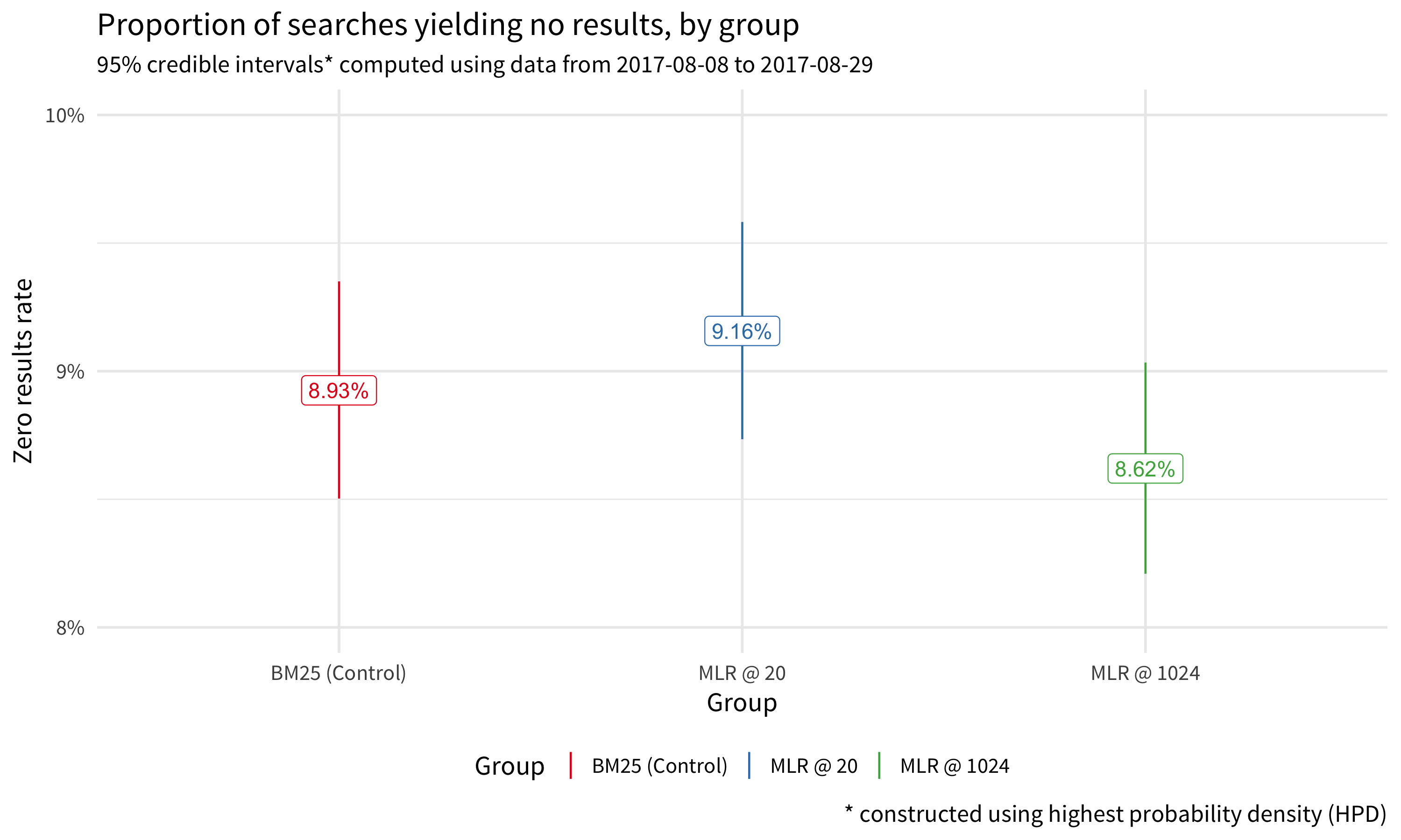
Figure 1: The zero results rate is not significantly different for the searches using MLR than the control group which used BM25 ranking.
Clickthrough rate
Currently, our primary assessment of performance with respect to relevance is users’ engagement with their search results as measured by their clickthrough rate – the proportion of searches where the user received some search results and clicked on at least one of them. Figure 2 shows that users who received MLR results were slightly more likely to engage with those results than users who received results retrieved via BM25.
set.seed(0)
ctr <- serp_clicks[valid == TRUE, list(clickthrough = any(event == "click"), max_hits = max(hits_returned, na.rm = TRUE)),
                   by = c("group_id", "session_id", "search_id")] %>%
  # filter out searches with 0 results
  .[max_hits > 0, list(searches = .N, clickthroughs = sum(clickthrough)), by = "group_id"] %>%
  { cbind(group = .$group_id, binom::binom.bayes(.$clickthroughs, .$searches)) }

ggplot(ctr, aes(x = group, color = group, y = mean, ymin = lower, ymax = upper)) +
  geom_linerange() +
  geom_label(aes(label = sprintf("%.2f%%", 100 * mean)), show.legend = FALSE) +
  scale_color_brewer(palette = "Set1") +
  scale_y_continuous(labels = scales::percent_format()) +
  labs(
    x = "Group", color = "Group", y = "Clickthrough rate",
    title = "Proportion of searches where the user clicked a result, by group",
    subtitle = sprintf("95%% credible intervals* computed using data from %s to %s", min(serp_clicks$date), max(serp_clicks$date)),
    caption = "* constructed using highest probability density (HPD)"
  ) +
  wmf::theme_min(14, ifelse(is_html(), "Source Sans Pro", "Gill Sans"))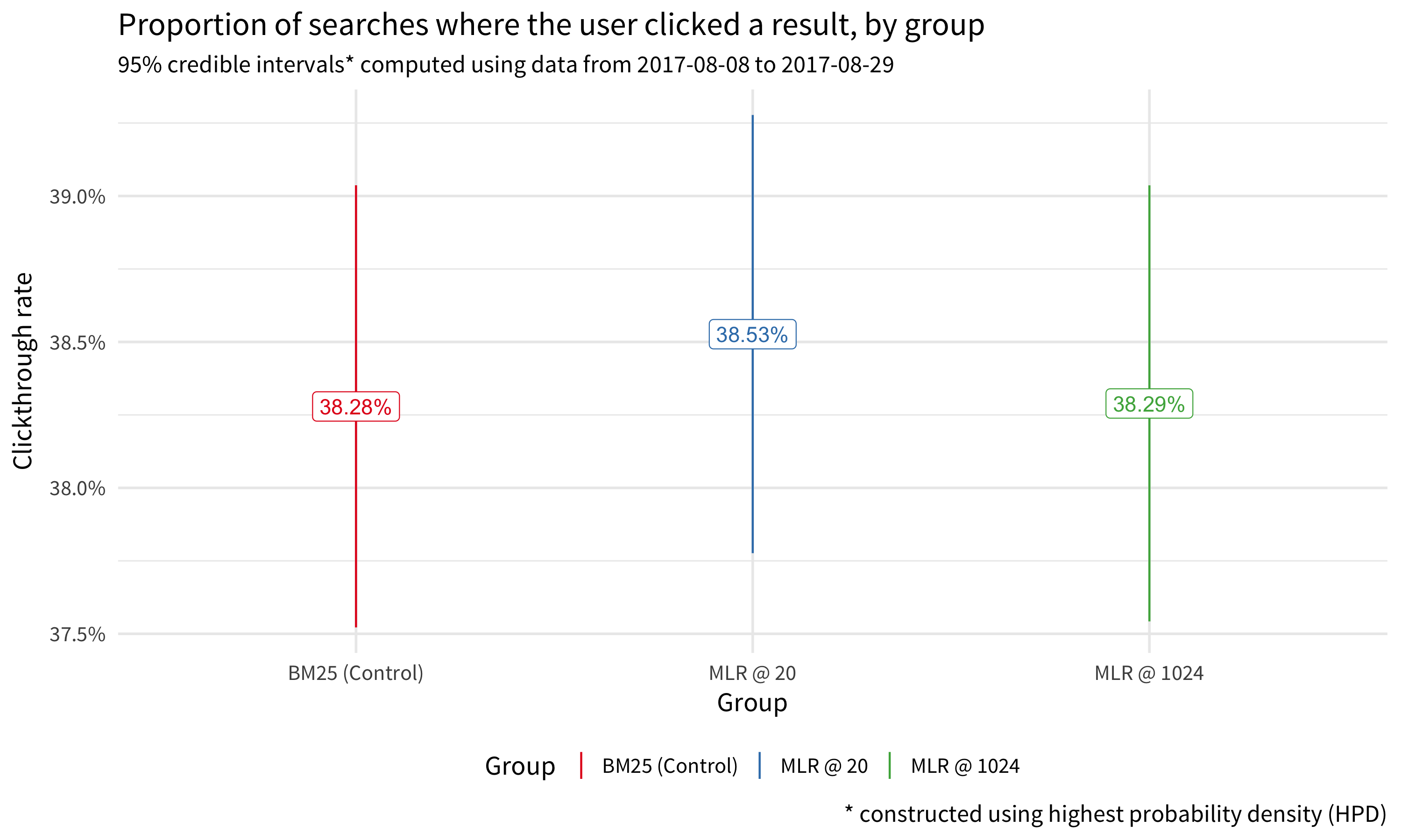
Figure 2: MLR@20 experimental group had slightly higher engagement with their MLR-provided search results than the control group had with their BM25-provided search results, but not by much.
Position of first click
Another way to assess the relevance quality of search results is to look at which results users clicked first. Specifically, one could assume that the first result a user clicks on is the one they judged to be the most relevant and that the position of the first clicked result gives an insight into how well the ranker performs.
set.seed(0)
first_click <- serp_clicks %>%
  as.data.frame %>%
  keep_where(event == "click", valid == TRUE) %>%
  group_by(group_id, session_id, search_id) %>%
  dplyr::top_n(1, ts) %>%
  group_by(group_id, position) %>%
  dplyr::tally() %>%
  mutate(
    position = dplyr::if_else(
      position < 4,
      purrr::map_chr(position + 1, toOrdinal::toOrdinal),
      "5+"
    ),
    position = factor(position, c("1st", "2nd", "3rd", "4th", "5+"))
  ) %>%
  group_by(group_id, position) %>%
  summarize(n = sum(n)) %>%
  mutate(total = sum(n)) %>%
  ungroup %>%
  { cbind(., binom::binom.bayes(.$n, .$total)) }

ggplot(first_click, aes(x = position, y = mean, fill = group_id)) +
  geom_bar(stat = "identity", position = position_dodge(width = 0.9), color = "white") +
  geom_errorbar(aes(ymin = lower, ymax = upper), position = position_dodge(width = 0.9), width = 0.2) +
  geom_text(
    aes(label = sprintf("%.1f%%", 100 * mean), y = upper + 0.01),
    position = position_dodge(width = 0.9),
    vjust = "bottom"
  ) +
  scale_fill_brewer(palette = "Set1") +
  scale_y_continuous(labels = scales::percent_format()) +
  labs(
    x = "Position", y = "Proportion of searches with a clickthrough",
    fill = "Group", title = "Position of first clicked result, by group",
    subtitle = "Error bars indicate 95% credible interval (via HPD)"
  ) +
  wmf::theme_min(14, ifelse(is_html(), "Source Sans Pro", "Gill Sans"))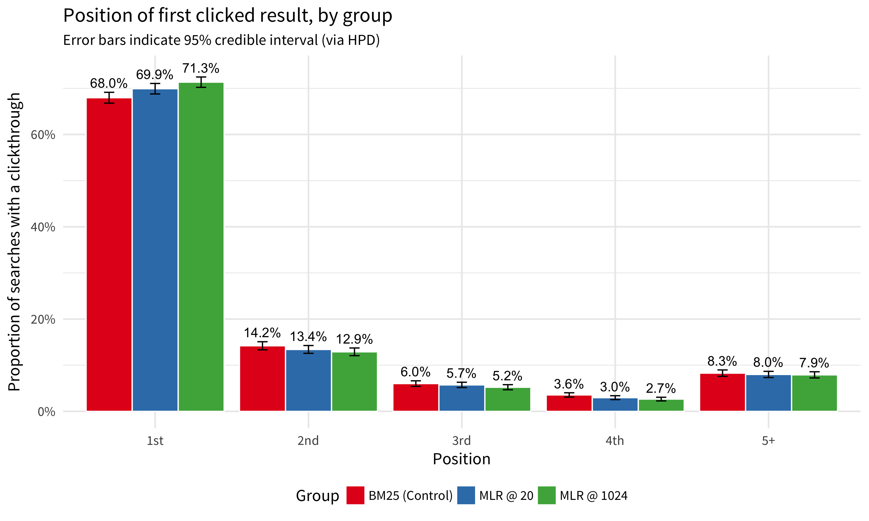
Figure 3: While users in general tend to click on the first search result first, users in the groups with MLR-provided results were slightly more likely than users in the control group with BM25-provided results.
Figure 3 shows that that a slightly higher proportion of users in the MLR groups clicked on the first search result first than the users in the control group. Focusing on first position specifically, we found that:
- The difference between control group and MLR@20 group was not statistically significant.
- The difference between control group and MLR@1024 group was statistically significant.
- The difference between MLR@20 and MLR@1024 groups was not statistically significant.
Page visit times
When a user is enrolled into search analytics tracking, we use survival analysis to estimate how long they keep clicked search results open. While the intent of the user making the search can vary and the time spent on visited pages varies with that – for example, we cannot expect the user who searched for “barack obama birthdate” to stay on Barack Obama’s Wikipedia article for more than a few seconds after seeing the birthdate in the infobox – this is still a window into potential differences in users’ perception of the results. Specifically, Figure 4 shows that users who navigated to articles from search with MLR results were slightly more likely to stay on those articles longer, perhaps because they were more relevant.
temp <- page_visits[valid == TRUE, {
  if (any(.SD$event == "checkin")) {
    last_checkin <- max(.SD$checkin, na.rm = TRUE)
    idx <- which(checkins > last_checkin)
    if (length(idx) == 0) idx <- 16
    next_checkin <- checkins[min(idx)]
    status <- ifelse(last_checkin == 420, 0, 3)
    data.table::data.table(
      `last check-in` = as.integer(last_checkin),
      `next check-in` = as.integer(next_checkin),
      status = as.integer(status)
    )
  }
}, by = c("group_id", "session_id", "search_id")]
surv <- survival::Surv(
  time = temp$`last check-in`,
  time2 = temp$`next check-in`,
  event = temp$status,
  type = "interval"
)
fit <- survival::survfit(surv ~ temp$group_id)
km <- survminer::ggsurvplot(
  fit, data = temp,
  palette = "Set1", conf.int = FALSE,
  ggtheme = wmf::theme_min(14, ifelse(is_html(), "Source Sans Pro", "Gill Sans")),
  title = "How long users stay on clicked results, by group",
  subtitle = "Kaplan–Meier curve of estimated survival probability",
  xlab = "Time (s)", ylab = "Probability of visited page staying open this long"
)
km$plot <- km$plot + scale_y_continuous(labels = scales::percent_format())
print(km)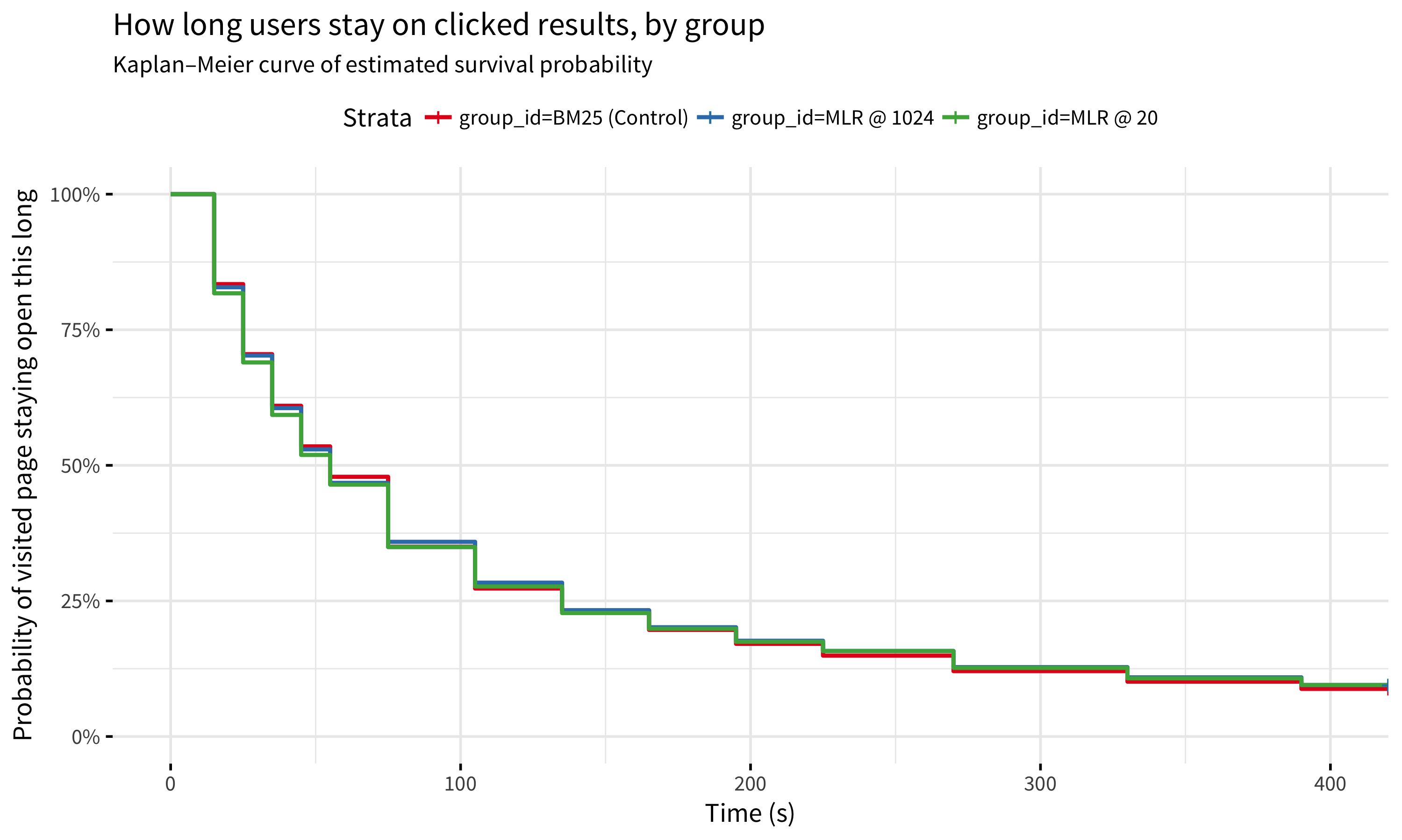
Figure 4: Users were slightly more likely to stay on MLR-provided pages longer than users who clicked on BM25-provided results.
Pagination navigation
Figure 5 shows that users did not explore the various pages of search results presented to them and mostly stayed on the first page containing the top 20 (or top 15) results. It also shows that there were no significant differences between the groups.
set.seed(0)
explored <- serp_clicks %>%
  as.data.frame %>%
  keep_where(event == "searchResultPage" & hits_returned > 0, valid == TRUE) %>%
  group_by(group_id, session_id, search_id) %>%
  summarize(explored = max(offset, na.rm = TRUE) > 0) %>%
  group_by(group_id) %>%
  summarize(searches = n(), explored = sum(explored)) %>%
  { cbind(group = .$group_id, binom::binom.bayes(.$explored, .$searches)) }

ggplot(explored, aes(x = group, color = group, y = mean, ymin = lower, ymax = upper)) +
  geom_linerange() +
  geom_label(aes(label = sprintf("%.2f%%", 100 * mean)), show.legend = FALSE) +
  scale_color_brewer(palette = "Set1") +
  scale_y_continuous(labels = scales::percent_format()) +
  labs(
    x = "Group", color = "Group", y = "Proportion of searches that yielded some results",
    title = "Proportion of searches where the user viewed additional results, by group",
    subtitle = sprintf("95%% HPD intervals computed using data from %s to %s", min(serp_clicks$date), max(serp_clicks$date)),
    caption = "By tracking the offset values, we are able to know when the user clicked on page 2 or 3 of search results."
  ) +
  wmf::theme_min(14, ifelse(is_html(), "Source Sans Pro", "Gill Sans"))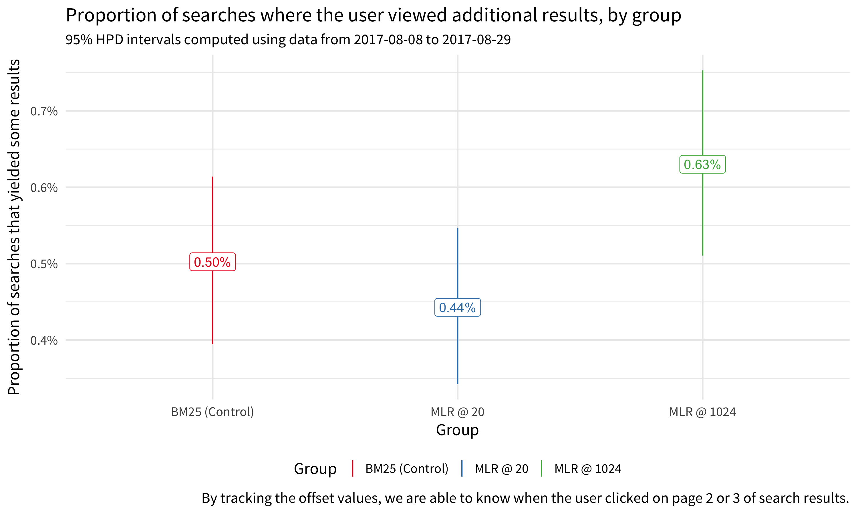
Figure 5: Users rarely clicked past the first page of search results and primarily saw the top 20 (or top 15) results. There were no significant differences in the proportions of sessions (which yielded search results) between the three groups.
Interleaved test
Preference
In the interleaved setting where users saw a mix of search results from two different ranking functions, we observed a slight but statistically insignificant preference for results from MLR@20 and specifically from MLR@1024. The daily preferences in Figure 6 show a count of days in which users preferred results from team “A” versus results from team “B”. For example, there were 6-8 days in which users preferred results from BM25 and 13-15 days in which users preferred results from MLR with a rescore window of 1024. Looking at the overall preferences in Figure 7, users showed a slightly higher preferences for MLR@1024 results over BM25 results than for MLR@20 results over BM25 results, but when we presented them with MLR results from both rescore windows, there was practically no preference.
events <- interleaved[
  !is.na(team) & team != "" & event == "visitPage" & valid == TRUE,
  c("date", "group_id", "session_id", "search_id", "team"),
  with = TRUE
]
events <- events[order(events$date, events$group_id, events$session_id, events$search_id, events$team), ]
pref_daily <- events[, j = list(
  "Sampling sessions" = wmf::interleaved_preference(paste(.SD$session_id), .SD$team),
  "Sampling searches" = wmf::interleaved_preference(paste(.SD$session_id, .SD$search_id), .SD$team)
), by = c("date", "group_id")] %>%
  tidyr::gather(method, observed, -c(date, group_id))
pref_overall <- events[, j = list(
  "Sampling sessions" = wmf::interleaved_preference(paste(.SD$session_id), .SD$team),
  "Sampling searches" = wmf::interleaved_preference(paste(.SD$session_id, .SD$search_id), .SD$team)
), by = c("group_id")] %>%
tidyr::gather(method, observed, -c(group_id))data.table::setDTthreads(4) # not sure if this actually even helps
set.seed(42)
prefs_by_session <- events[, {
preferences <- vapply(1:m, function(i) {
set.seed(i)
n <- data.table::uniqueN(.SD$session_id)
resampled <- split(.SD, .SD$session_id)[sample.int(n, n, replace = TRUE)]
names(resampled) <- 1:n
resampled %>%
dplyr::bind_rows(.id = "sample") %>%
group_by(session_id) %>%
mutate(sample_id = paste(session_id, as.numeric(factor(sample)), sep = "-")) %>%
ungroup %>%
{ wmf::interleaved_preference(.$sample_id, .$team) }
}, 0.0)
data.frame(sample = 1:m, preference = preferences, method = "Sampling sessions", stringsAsFactors = FALSE)
}, by = c("date", "group_id")]
prefs_by_search <- events[, {
preferences <- vapply(1:m, function(i) {
set.seed(i)
n <- data.table::uniqueN(.SD[, c("session_id", "search_id"), with = TRUE])
resampled <- split(.SD, paste0(.SD$session_id, .SD$search_id))[sample.int(n, n, replace = TRUE)]
names(resampled) <- 1:n
resampled %>%
dplyr::bind_rows(.id = "sample") %>%
group_by(session_id, search_id) %>%
mutate(sample_id = paste(session_id, search_id, as.numeric(factor(sample)), sep = "-")) %>%
ungroup %>%
{ wmf::interleaved_preference(.$sample_id, .$team) }
}, 0.0)
data.frame(sample = 1:m, preference = preferences, method = "Sampling searches", stringsAsFactors = FALSE)
}, by = c("date", "group_id")]
prefs <- rbind(prefs_by_session, prefs_by_search)
daily <- prefs %>%
group_by(date, group_id, method) %>%
summarize(
lower = quantile(preference, 0.025, na.rm = TRUE),
upper = quantile(preference, 0.975, na.rm = TRUE)
) %>%
ungroup %>%
left_join(pref_daily, by = c("date", "group_id", "method")) %>%
mutate(preferred = dplyr::if_else(observed > 0, "A", "B")) %>%
group_by(group_id, method, preferred) %>%
arrange(date) %>%
mutate(counter = cumsum(!is.na(date))) %>%
ungroup
overall <- prefs %>%
group_by(group_id, method, date) %>%
summarize(
lower95 = quantile(preference, 0.025, na.rm = TRUE),
lower80 = quantile(preference, 0.1, na.rm = TRUE),
upper95 = quantile(preference, 0.975, na.rm = TRUE),
upper80 = quantile(preference, 0.9, na.rm = TRUE),
) %>%
summarize(
lower95 = median(lower95, na.rm = TRUE),
upper95 = median(upper95, na.rm = TRUE),
lower80 = median(lower80, na.rm = TRUE),
upper80 = median(upper80, na.rm = TRUE)
) %>%
ungroup %>%
left_join(pref_overall, by = c("group_id", "method"))ggplot(keep_where(daily, !is.na(observed)), aes(x = date, y = observed)) +
geom_hline(yintercept = 0, linetype = "dashed") +
geom_ribbon(aes(ymin = lower, ymax = upper), alpha = 0.25) +
geom_line() +
geom_segment(
aes(xend = date, yend = ifelse(preferred == "A", 0.275, -0.275), color = preferred),
linetype = "dotted"
) +
geom_point(aes(color = preferred)) +
geom_text(
aes(y = ifelse(preferred == "A", 0.3, -0.3), label = counter, color = preferred),
show.legend = FALSE, fontface = "bold"
) +
scale_color_brewer(palette = "Set1") +
facet_grid(method ~ group_id) +
labs(
x = "Date", y = ifelse(is_html(), "B ← Preference → A", "B < Preference > A"),
title = "Preference for results from two rankers, daily by group",
subtitle = "Showing counts of how many times users preferred one ranking over the other",
caption = "95% confidence intervals were bootstrapped using two different sampling approaches"
) +
wmf::theme_facet(14, ifelse(is_html(), "Source Sans Pro", "Gill Sans"))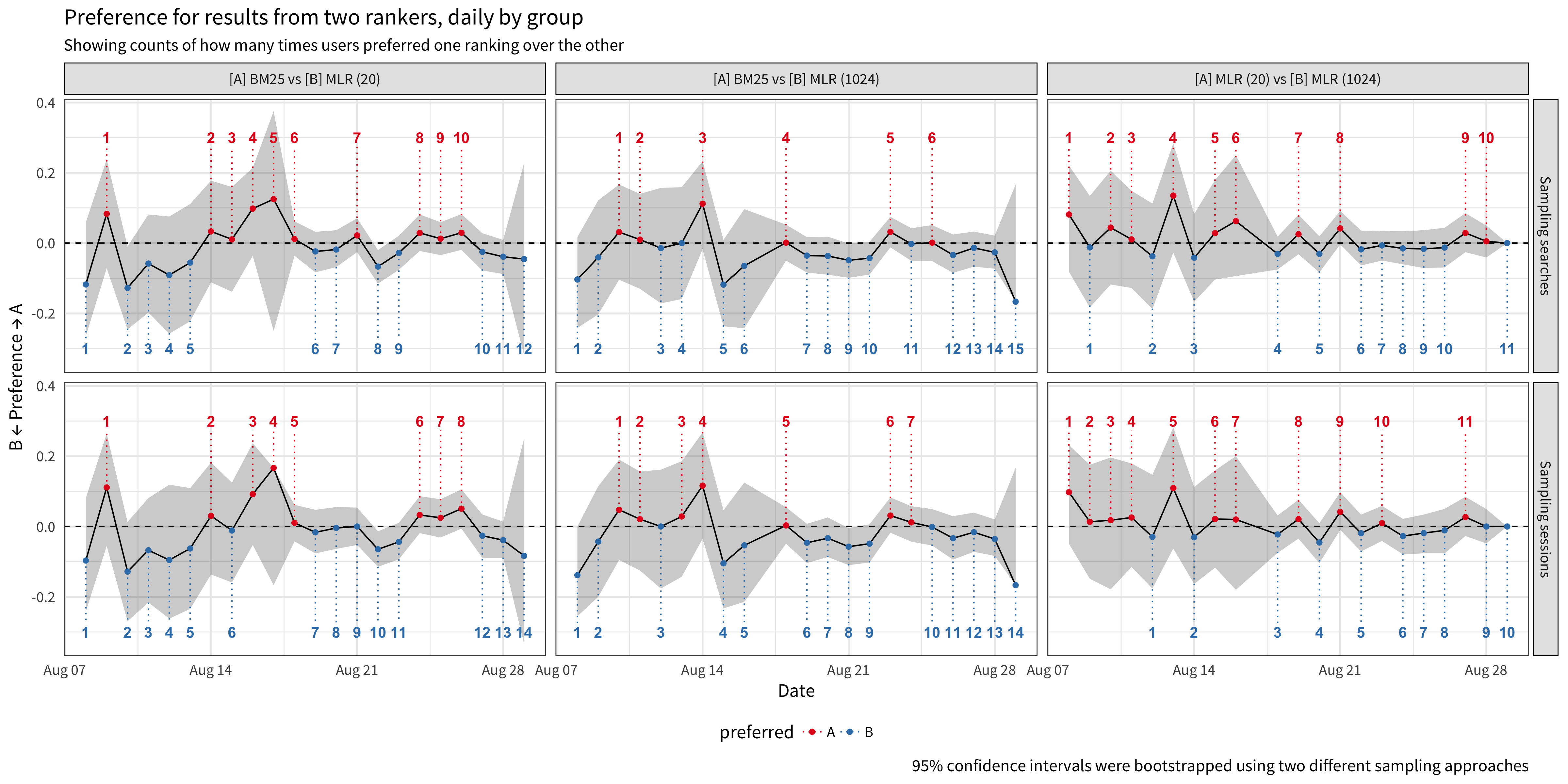
Figure 6: While the preferences for ranking functions were not significantly higher or lower (the 95% bootstrapped confidence intervals cover 0 – no preference) on a daily basis, there were more days when the users showed a slight preference for MLR results with the 1024-rescore window.
ggplot(
  mutate(overall, method = sub("\\s", "\n", method)),
  aes(x = method, y = observed)
) +
  geom_hline(yintercept = 0, linetype = "dashed") +
  geom_linerange(aes(ymin = lower95, ymax = upper95), size = 0.5) +
  geom_linerange(aes(ymin = lower80, ymax = upper80), size = 1.5) +
  geom_label(aes(label = sprintf("%.4f", observed))) +
  facet_wrap(~ group_id) +
  labs(
    x = "Bootstrap approach", y = ifelse(is_html(), "B ← Preference → A", "B < Preference > A"),
    title = "Preference for results from two rankers, by group",
    caption = "80% (thick) and 95% (thin) confidence intervals were bootstrapped using two different sampling approaches"
  ) +
  wmf::theme_facet(14, ifelse(is_html(), "Source Sans Pro", "Gill Sans"))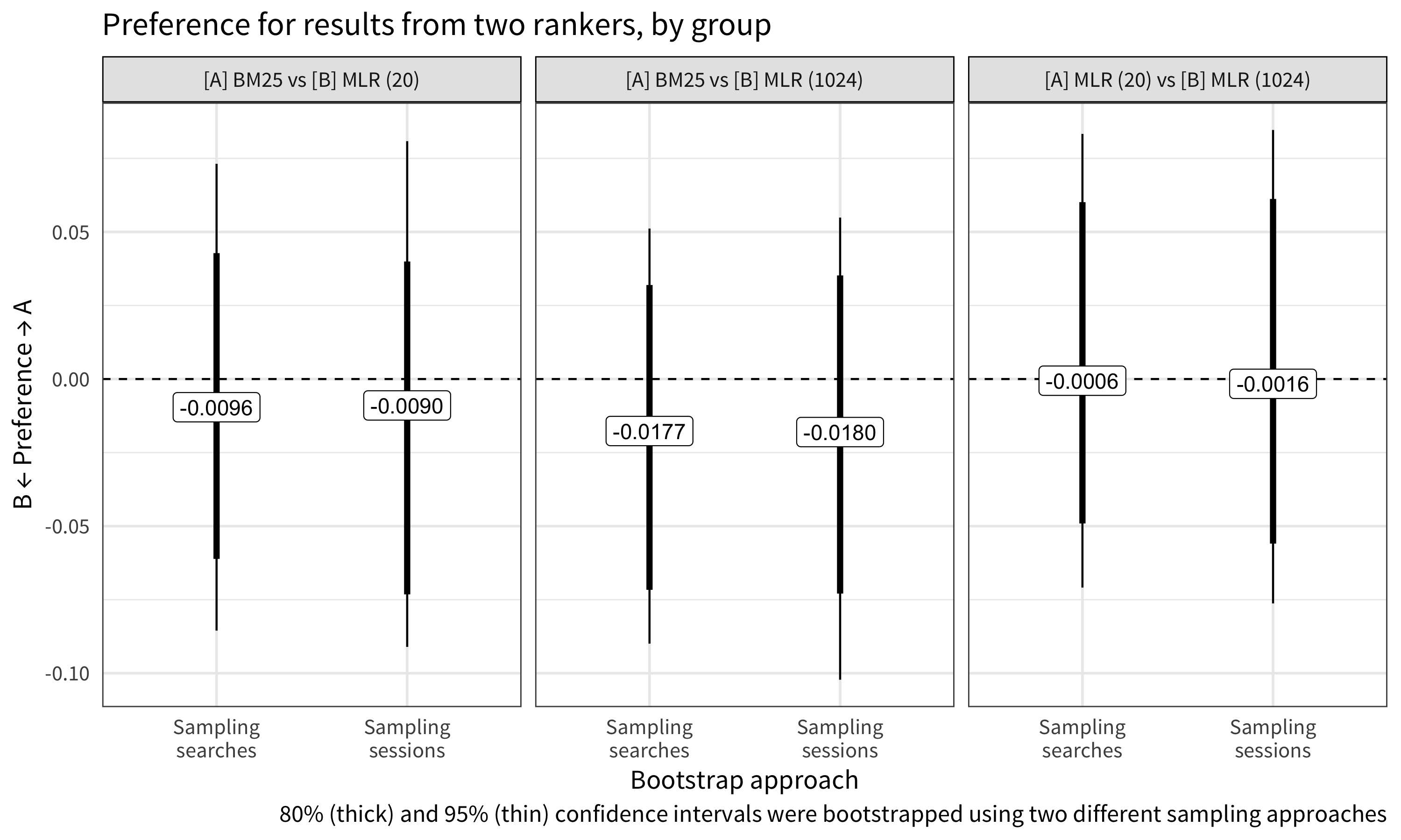
Figure 7: Overall, there were not statistically significant differences in preferences (the 95% bootstrapped confidence intervals cover 0 – no preference), although the results suggest that users showed a slight preference for MLR results with the 1024-rescore window.
Page visit times
As mentioned before, observing how long users stay on visited pages is a way to gauge the relevance of the search results in the context of trying to find a specific article to read. Figure 8 shows that compared to the BM25-provided results, pages that were provided by MLR had a higher probability of being open longer – indicating that users were staying longer on those clicked results. Between the two sets of MLR-provided results, pages that were provided by the 1024-rescore window MLR had a higher probability of staying open longer.
temp <- interleaved[!is.na(team) & team != "" & valid == TRUE, {
  if (any(.SD$event == "checkin")) {
    last_checkin <- max(.SD$checkin, na.rm = TRUE)
    idx <- which(checkins > last_checkin)
    if (length(idx) == 0) idx <- 16
    next_checkin <- checkins[min(idx)]
    status <- ifelse(last_checkin == 420, 0, 3)
    data.table::data.table(
      `last check-in` = as.integer(last_checkin),
      `next check-in` = as.integer(next_checkin),
      status = as.integer(status),
      team = .SD$team[1]
    )
  }
}, by = c("group" = "group_id", "session_id", "search_id")] %>%
  as.data.frame
temp$group %<>% factor(
  c("[A] BM25 vs [B] MLR (20)", "[A] BM25 vs [B] MLR (1024)", "[A] MLR (20) vs [B] MLR (1024)"),
  c("1: BM25 vs LTR (20)", "2: BM25 vs LTR (1024)", "3: LTR (20) vs LTR (1024)")
)
surv <- survival::Surv(
  time = temp$`last check-in`,
  time2 = temp$`next check-in`,
  event = temp$status,
  type = "interval"
)
fit <- survival::survfit(surv ~ temp$group + temp$team)
km <- survminer::ggsurvplot(
  fit, data = temp, palette = "Dark2",
  title = "How long users stay on each team's results",
  subtitle = "Kaplan–Meier curve of estimated survival probability",
  xlab = "Time (s)", ylab = "Probability of visited page staying open this long"
)
km$plot <- km$plot +
  scale_y_continuous(labels = scales::percent_format()) +
  scale_x_continuous(labels = function(x) {
    mins <- floor(x / 60); secs <- x %% 60
    labs <- sprintf("%.0fm %.0fs", mins, secs)
    labs[mins == 0] <- sprintf("%.0fs", secs[mins == 0])
    labs[secs == 0] <- sprintf("%.0fm", mins[secs == 0])
    return(labs)
  }, breaks = c(0.5, 1:7) * 60) +
  facet_wrap(~ group) +
  wmf::theme_facet(14, ifelse(is_html(), "Source Sans Pro", "Gill Sans"))
print(km)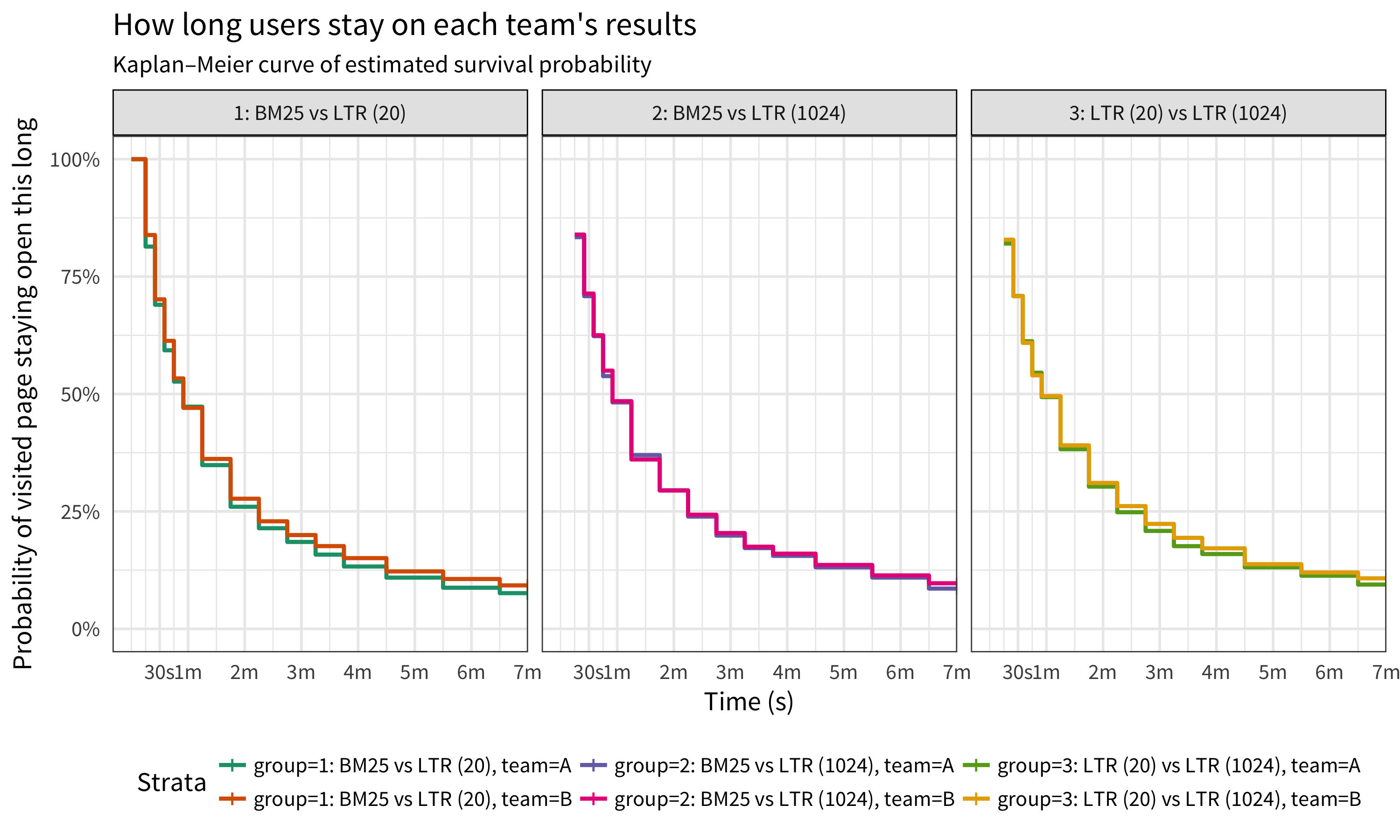
Figure 8: Compared to the BM25-provided results, pages that were provided by MLR had a higher probability of being open longer – indicating that users were staying longer on those clicked results. Between the two sets of MLR-provided results, pages that were provided by the 1024-rescore window MLR had a higher probability of staying open.
Conclusion
While we did not see overwhelming evidence that LTR is better than the status quo, we saw results that indicate a slight improvement. MLR@20’s clikthrough rate was slightly higher (although not statistically significantly higher), users preferred LTR over BM25 in the interleaved results more often than the other way, and overall there is a slight preference for LTR results over BM25 results. We did observe that MLR@20 users were statistically significantly more likely to click on the first search result first than users in the control group were to click on theirs.
Discussion
Regarding the rescore window, 1024 isn’t incredibly expensive compared to 20. It costs more, but it doesn’t seem prohibitive. In the load tests with rescore windows up to 4096, it was all fine. The benefit we would get from a larger rescore window is the ability to pull things up from further down in the retrieval query phase. The theory is that there are plenty of good things down there, and if we allow the LTR to reach down that far it will find them. This gives new information to the DBN, which hopefully builds a feedback loop where the LTR brings in some new result types from further down that it thinks are good, users evaluate them, and then the DBN learns new labels based on those to inform the next model we build.
Acknowledgement
We would like to thank our colleague Chelsy Xie for her review of this report.
References
Allaire, J., Cheng, J., Xie, Y., McPherson, J., Chang, W., Allen, J., et al. (2016). Rmarkdown: Dynamic documents for r. http://rmarkdown.rstudio.com
Bache, S. M., & Wickham, H. (2014). Magrittr: A forward-pipe operator for r. https://CRAN.R-project.org/package=magrittr
Bernhardson, E., Causse, D., Jones, T., Popov, M., & Tankersley, D. (2016). Improving search result relevancy on wikipedia with bm25 ranking. https://wikimedia-research.github.io/Discovery-Search-Test-BM25/
Bernhardson, E., Causse, D., Jones, T., Tankersley, D., & Xie, C. (2017). Second bm25 a/b test analysis. https://wikimedia-research.github.io/Discovery-Search-2ndTest-BM25_jazhth/
Chapelle, O., & Zhang, Y. (2009). A dynamic bayesian network click model for web search ranking. New York, New York, USA: ACM.
Chapelle, O., Joachims, T., Radlinski, F., & Yue, Y. (2012). Large-scale validation and analysis of interleaved search evaluation. ACM Trans. Inf. Syst., 30(1), 6:1–6:41. doi:10.1145/2094072.2094078
Dowle, M., & Srinivasan, A. (2017). Data.table: Extension of ‘data.frame‘. https://CRAN.R-project.org/package=data.table
Keyes, O., & Popov, M. (2017). Wmf: R code for wikimedia foundation internal usage. https://phabricator.wikimedia.org/diffusion/1821/
Ooms, J. (2014). The jsonlite package: A practical and consistent mapping between json data and r objects. arXiv:1403.2805 [stat.CO]. https://arxiv.org/abs/1403.2805
R Core Team. (2016). R: A language and environment for statistical computing. Vienna, Austria: R Foundation for Statistical Computing. https://www.R-project.org/
Wickham, H. (2009). Ggplot2: Elegant graphics for data analysis. Springer-Verlag New York. http://ggplot2.org
Wickham, H. (2017). Tidyr: Easily tidy data with ’spread()’ and ’gather()’ functions. https://CRAN.R-project.org/package=tidyr
Wickham, H., & Francois, R. (2016). Dplyr: A grammar of data manipulation. https://CRAN.R-project.org/package=dplyr