Swap2and3 Search Test Analysis
Erik Bernhardson
Senior Software Engineer, Wikimedia FoundationTrey Jones
Senior Software Engineer, Wikimedia FoundationChelsy Xie
Data Analyst, Wikimedia FoundationMikhail Popov
Data Analyst, Wikimedia FoundationDeb Tankersley
Product Manager (Analysis, Search Frontend), Wikimedia Foundation14 September 2017
Abstract
Wikimedia Technology’s Search Platform team ran an A/B test from April 7 to April 25, 2016 to see how much our users care about the position of the result vs the actual content of the result by swapping the second and third search results. We found that position 2 had a higher clickthrough rate than position 3 in both groups, but the clickthrough rate of the 3rd result was higher in the test group than in the control group. We also found that test group users were less likely to click on the 2nd result first than the control group and were more likely to click on the 3rd result first. Based on the resultsof this analysis, we think that both position and quality matter in user behavior, but with different weights. Further experiments are needed to figure out the quantitative relationship between user behavior and these two factors.
{ RMarkdown Source | Analysis Codebase }
Data
data1 <- data1 %>% filter(
  (event_action == 'searchResultPage' & !is.na(event_hitsReturned)) |
  (event_action == 'click' & !is.na(event_position) & event_position > -1) |
  (event_action == 'visitPage' & !is.na(event_pageViewId)) |
  (event_action == 'checkin' & !is.na(event_checkin) & !is.na(event_pageViewId))
)
data1$event_subTest[is.na(data1$event_subTest)] <- "Control"
data1 <- data1[!duplicated(data1$id), ]
data1$date <- lubridate::ymd(substr(data1$timestamp, 1,8))
data1 <- data1 %>%
  group_by(date, event_subTest, event_mwSessionId, event_searchSessionId) %>%
  filter("searchResultPage" %in% event_action) %>%
  ungroup %>% as.data.frame() # remove search_id without SERP asscociated
## 6474 out of 301603 search sessions fall into both control and test group... Delete those sessions
temp <- data1 %>% group_by(event_searchSessionId) %>% summarise(count=length(unique(event_subTest)))
data1 <- data1[data1$event_searchSessionId %in% temp$event_searchSessionId[temp$count==1], ]; rm(temp)| Test group | Search sessions | Events recorded |
|---|---|---|
| Control | 157,713 | 675,211 |
| swap2and3 | 137,416 | 483,407 |
| Total | 295,129 | 1,158,618 |
As in another A/B test analysis we did before, there is an issue with the event logging that when a user goes to the next page of search results or clicks the Back button after visiting a search result, a new page ID is generated for the search results page. The page ID is how we connect click events to search result page events. For this analysis, we de-duplicated by connecting search engine results page (searchResultPage) events that have the exact same search query, and then connected click events together based on the searchResultPage connectivity.
# De-duplication
temp <- data1 %>%
  filter(event_action == "searchResultPage") %>%
  group_by(event_mwSessionId, event_searchSessionId, event_query) %>%
  mutate(new_page_id = min(event_pageViewId)) %>%
  ungroup %>%
  select(c(event_pageViewId, new_page_id)) %>%
  distinct
data1 <- left_join(data1, temp, by = "event_pageViewId"); rm(temp)
data1$new_page_id[is.na(data1$new_page_id)] <- data1$event_pageViewId[is.na(data1$new_page_id)]
temp <- data1 %>%
  filter(event_action == "searchResultPage") %>%
  arrange(new_page_id, timestamp) %>%
  mutate(dupe = duplicated(new_page_id, fromLast = FALSE)) %>%
  select(c(id, dupe))
data1 <- left_join(data1, temp, by = "id"); rm(temp)
data1$dupe[data1$event_action != "searchResultPage"] <- FALSE
data1 <- data1[!data1$dupe & !is.na(data1$new_page_id), ] %>%
  select(-c(event_pageViewId, dupe)) %>%
  rename(page_id = new_page_id) %>%
  arrange(date, event_mwSessionId, event_searchSessionId, page_id, desc(event_action), timestamp)
# Summarize on a page-by-page basis for each SERP:
searches <- data1 %>%
  group_by(`test group` = event_subTest, event_mwSessionId, event_searchSessionId, page_id) %>%
  filter("searchResultPage" %in% event_action) %>% # keep only searchResultPage and click
  summarize(timestamp = timestamp[1],
            results = ifelse(event_hitsReturned[1] > 0, "some", "zero"),
            clickthrough = "click" %in% event_action,
            `no. results clicked` = length(unique(event_position))-1,
            `first clicked result's position` = ifelse(clickthrough, na.omit(event_position)[1][1], NA), #There are some search with click, but position is NA
            `Clicked on position 2` = 2 %in% event_position,
            `Clicked on position 3` = 3 %in% event_position
            ) %>%
arrange(timestamp)| Test group | Search sessions | Searches recorded | Events recorded |
|---|---|---|---|
| Control | 157,713 | 279,749 | 599,925 |
| swap2and3 | 137,416 | 204,167 | 438,227 |
| Total | 295,129 | 483,916 | 1,038,152 |
# Summarize on a page-by-page basis for each visitPage:
clickedResults <- data1 %>%
  group_by(test_group = event_subTest, event_mwSessionId, event_searchSessionId, page_id) %>%
  filter("visitPage" %in% event_action) %>% #only checkin and visitPage action
  summarize(timestamp = timestamp[1],
            position = na.omit(event_position)[1][1],
            dwell_time=ifelse("checkin" %in% event_action, max(event_checkin, na.rm=T), 0),
            scroll=sum(event_scroll)>0) %>%
  arrange(timestamp)
clickedResults$dwell_time[is.na(clickedResults$dwell_time)] <- 0
# 74148 clickedResults
clickedResults$status <- ifelse(clickedResults$dwell_time=="420", 1, 2)
Last but not least, it is worth noting that there are some issues in our data collecting process:
- Sometimes click events were not recorded while visitPage events were. This problem was solved in June 2016 by T137262. For this analysis, we treat both click event and visitPage event as a “click” when computing clickthrough rate, i.e. if there is either a click or a visitPage event in a session, we will say there is a clickthrough in that session.
- There were 6474 out of 301,603 search sessions falling into both control and test buckets. We deleted those sessions in the data cleansing step.
Results
Engagement
Firstly, we compared the overall clickthrough rate between control and test group. We’ve checked that there is no significant difference in zero results rate between these two groups. The plot below shows that for each session, the control group has a significantly higher engagement rate; for each search results page, the test group has higher engagement, but the difference is not significant.
# Compare overall CTR
# per session:
engagement_overall_session <- data1 %>%
  group_by(event_subTest, event_searchSessionId) %>%
  summarise(clickthrough = "click" %in% event_action|"visitPage" %in% event_action, results = sum(event_hitsReturned, na.rm=TRUE) > 0) %>%
  filter(results == TRUE) %>%
  group_by(event_subTest) %>%
  summarise(clicks = sum(clickthrough), session = n()) %>%
  cbind(binom:::binom.bayes(.$clicks, n=.$session)[, c("mean", "lower", "upper")])
  #knitr::kable(engagement_overall_session, format = "markdown", align = c("l", "r", "r", "r", "r", "r"))

# per SERP:
engagement_overall_serp <- searches %>%
  filter(results == "some") %>%
  group_by(`test group`) %>%
  summarise(clicks = sum(clickthrough), searches = n()) %>%
  cbind(binom:::binom.bayes(.$clicks, n=.$searches, tol=.Machine$double.eps^0.6)[, c("mean", "lower", "upper")])
  #knitr::kable(engagement_overall_serp, format = "markdown", align = c("l", "r", "r", "r", "r", "r"))

# plot
p_ctr_ses <- engagement_overall_session %>%
  ggplot(aes(x = 1, y = mean, color = event_subTest)) +
  geom_pointrange(aes(ymin = lower, ymax = upper), position = position_dodge(width = 1)) +
  scale_color_brewer("Test Group", palette = "Set1", guide = guide_legend(ncol = 2)) +
  scale_y_continuous(labels = scales::percent_format(), expand = c(0.01, 0.01)) +
  labs(x = NULL, y = "Clickthrough rate",
       title = "Proportion of sessions that include \n at least one click/visitPage event") +
  geom_text(aes(label = sprintf("%.1f%%", 100 * mean), y = upper + 0.0025, vjust = "bottom"),
            position = position_dodge(width = 1)) +
  theme(legend.position = "bottom")
p_ctr_serp <- engagement_overall_serp %>%
  ggplot(aes(x = 1, y = mean, color = `test group`)) +
  geom_pointrange(aes(ymin = lower, ymax = upper), position = position_dodge(width = 1)) +
  scale_color_brewer("Test Group", palette = "Set1", guide = guide_legend(ncol = 2)) +
  scale_y_continuous(labels = scales::percent_format(), expand = c(0.01, 0.01)) +
  labs(x = NULL, y = "Clickthrough rate",
       title = "Proportion of SERPs that include \n at least one click event") +
  geom_text(aes(label = sprintf("%.1f%%", 100 * mean), y = upper + 0.0025, vjust = "bottom"),
            position = position_dodge(width = 1)) +
  theme(legend.position = "bottom")
plot_grid(p_ctr_ses, p_ctr_serp)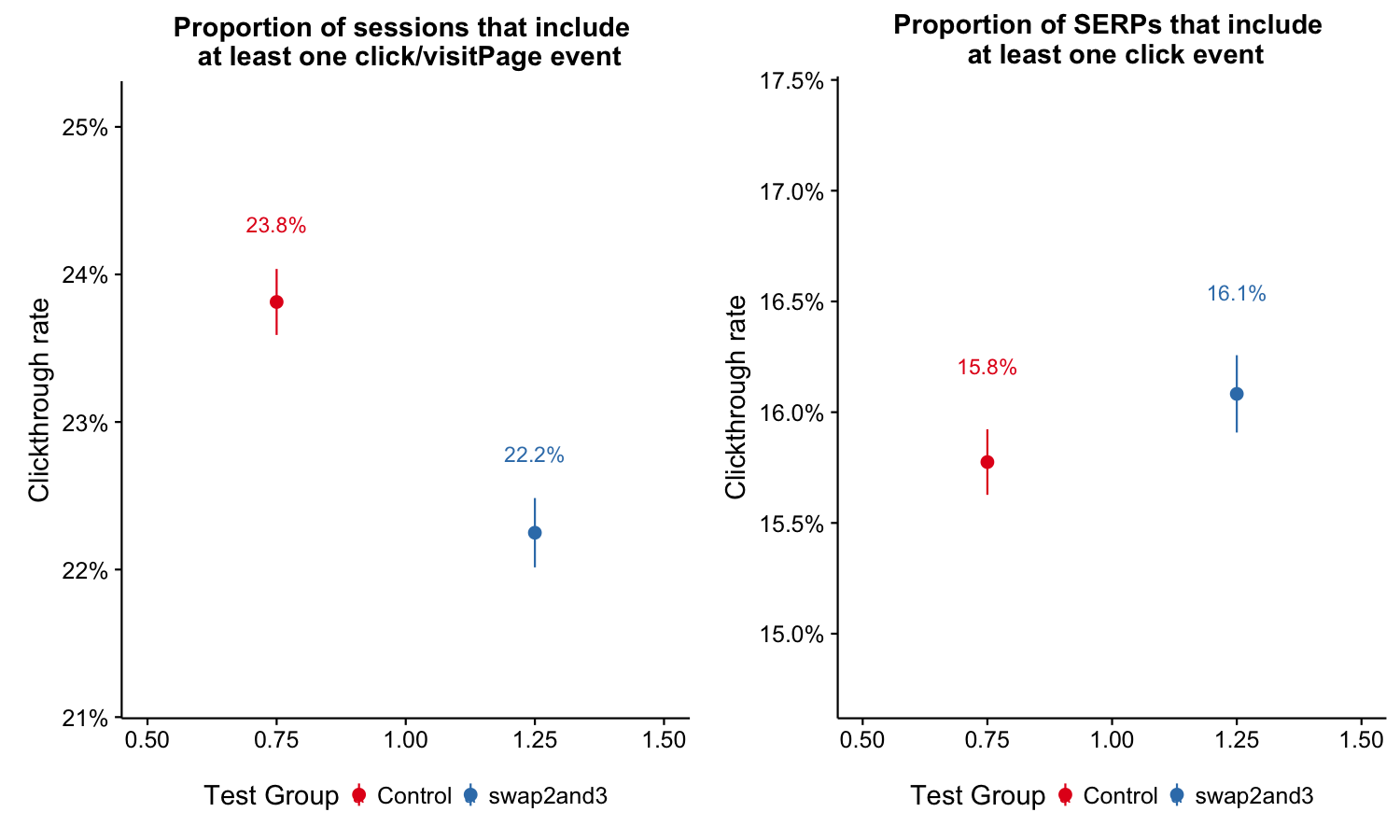
Figure 1: Proportion of sessions or searches that include at least one click/visitPage event by group.
Next, we compared the clickthrough rates in second and third position by test groups. All the differences in the graph below were significant. In both control and test groups, the clickthrough rates in position 2 were higher than position 3. When comparing the same position between groups, the engagement of the 3rd result in the test group was higher than that in the control group, but not as high as its counterpart, the 2nd result in the control group.
# Compare position 2 and 3
# per session, among all nonzero result session:
engagement_2and3_session <- data1 %>%
  group_by(event_subTest, event_searchSessionId) %>%
  summarise(clickthrough2 = 2 %in% event_position, clickthrough3 = 3 %in% event_position,
            clickthrough = "click" %in% event_action|"visitPage" %in% event_action, results = sum(event_hitsReturned, na.rm=TRUE) > 0) %>%
  filter(results == TRUE) %>%
  group_by(event_subTest) %>%
  summarise(clicked2 = sum(clickthrough2), clicked3 = sum(clickthrough3), session = n()) %>%
  cbind(binom:::binom.bayes(.$clicked2, n=.$session)[, c("mean", "lower", "upper")]) %>%
  rename(ctr2 = mean, lower2 = lower, upper2 = upper) %>%
  cbind(binom:::binom.bayes(.$clicked3, n=.$session)[, c("mean", "lower", "upper")]) %>%
  rename(ctr3 = mean, lower3 = lower, upper3 = upper)
# per SERP, among all nonzero result session:
engagement_2and3_serp <- searches %>%
  filter(results == "some") %>%
  group_by(`test group`) %>%
  summarise(clicked2 = sum(`Clicked on position 2`), clicked3 = sum(`Clicked on position 3`), searches = n()) %>%
  cbind(binom:::binom.bayes(.$clicked2, n=.$searches, tol=.Machine$double.eps^0.7)[, c("mean", "lower", "upper")]) %>%
  rename(ctr2 = mean, lower2 = lower, upper2 = upper) %>%
  cbind(binom:::binom.bayes(.$clicked3, n=.$searches, tol=.Machine$double.eps^0.7)[, c("mean", "lower", "upper")]) %>%
  rename(ctr3 = mean, lower3 = lower, upper3 = upper)

# plot
p_ctr23_ses <- engagement_2and3_session[, c("ctr2", "lower2", "upper2")] %>%
  rbind(setNames(engagement_2and3_session[, c("ctr3", "lower3", "upper3")], names(.))) %>%
  mutate(`test group` = c("Control_position2", "swap2and3_position2", "Control_position3", "swap2and3_position3")) %>%
  ggplot(aes(x = 1, y = ctr2, color = `test group`)) +
  geom_pointrange(aes(ymin = lower2, ymax = upper2), position = position_dodge(width = 1)) +
  scale_color_brewer("Test Group", palette = "Set1", guide = guide_legend(ncol = 2)) +
  scale_y_continuous(labels = scales::percent_format(), expand = c(0.01, 0.01)) +
  labs(x = NULL, y = "Clickthrough rate",
       title = "Proportion of sessions that include \n at least one click/visitPage event in position x") +
  geom_text(aes(label = sprintf("%.1f%%", 100 * ctr2), y = upper2 + 0.0025, vjust = "bottom"),
            position = position_dodge(width = 1)) +
  theme(legend.position = "bottom")
p_ctr23_serp <- engagement_2and3_serp[, c("ctr2", "lower2", "upper2")] %>%
  rbind(setNames(engagement_2and3_serp[, c("ctr3", "lower3", "upper3")], names(.))) %>%
  mutate(`test group` = c("Control - 2nd result", "swap2and3 - 2nd result", "Control - 3rd result", "swap2and3 - 3rd result")) %>%
  ggplot(aes(x = 1, y = ctr2, color = `test group`)) +
  geom_pointrange(aes(ymin = lower2, ymax = upper2), position = position_dodge(width = 1)) +
  scale_color_brewer("Test Group", palette = "Set1", guide = guide_legend(ncol = 2)) +
  scale_y_continuous(labels = scales::percent_format(), expand = c(0.01, 0.01)) +
  labs(x = NULL, y = "Clickthrough rate",
       title = "Proportion of SERPs that include \n at least one click event in position x") +
  geom_text(aes(label = sprintf("%.1f%%", 100 * ctr2), y = upper2 + 0.0025, vjust = "bottom"),
            position = position_dodge(width = 1)) +
  theme(legend.position = "bottom")
par(mar=c(1,1,1,1), oma=c(1,1,1,1))
plot_grid(p_ctr23_ses, p_ctr23_serp)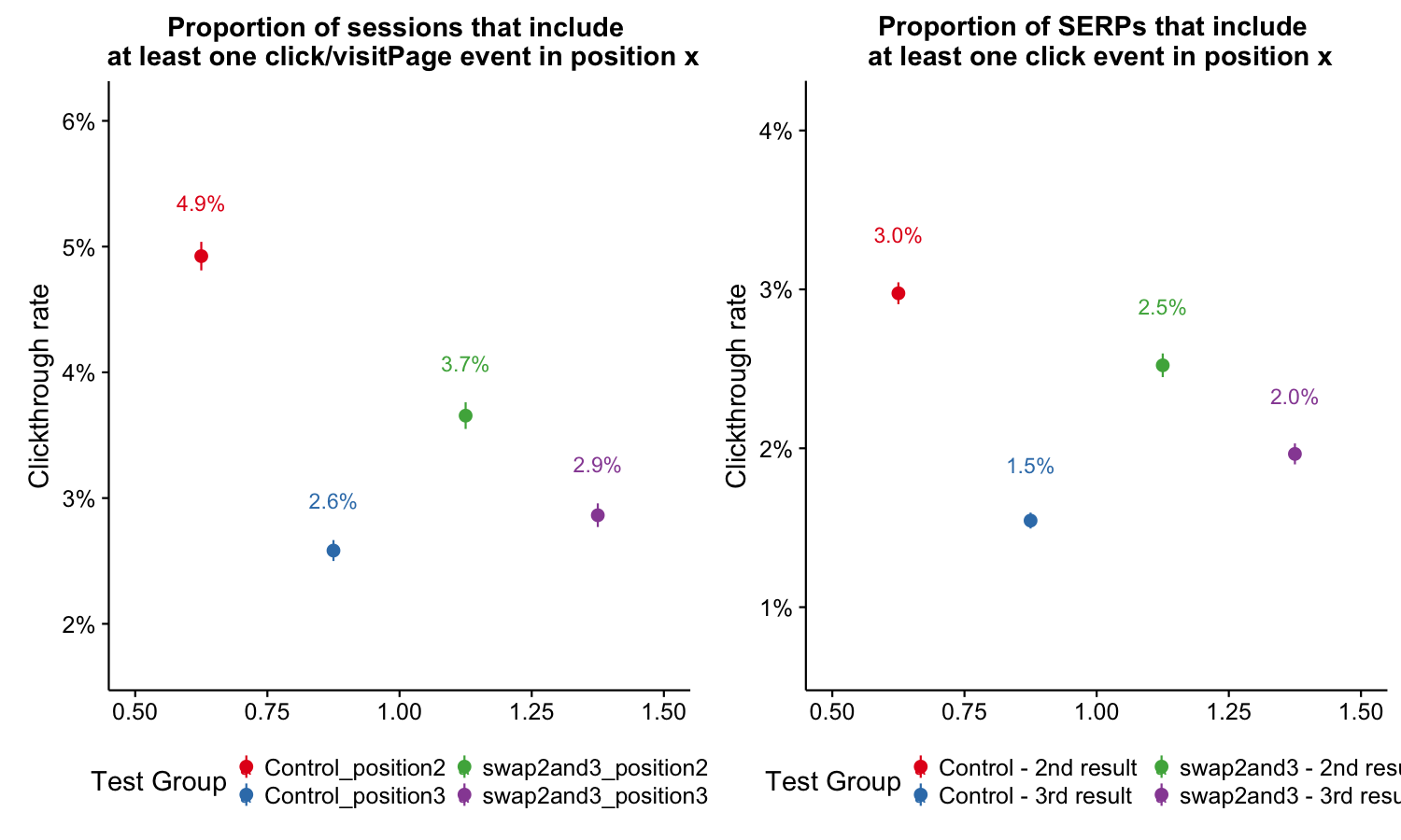
Figure 2: Proportion of sessions or searches that include at least one click/visitPage event by position and group.
First Clicked Result’s Position
We can see that test group users were less likely to click on the second result first than the control group, while they were more likely to click on the third result first. There is no significant difference in other positions.
safe_ordinals <- function(x) {
  return(vapply(x, toOrdinal::toOrdinal, ""))
}
first_clicked <- searches %>%
  filter(results == "some" & clickthrough & !is.na(`first clicked result's position`)) %>%
  mutate(`first clicked result's position` = ifelse(`first clicked result's position` < 5, safe_ordinals(`first clicked result's position`), "5th or higher")) %>%
  group_by(`test group`, `first clicked result's position`) %>%
  tally %>%
  mutate(total = sum(n), prop = n/total) %>%
  ungroup
temp <- as.data.frame(binom:::binom.bayes(first_clicked$n, n = first_clicked$total)[, c("mean", "lower", "upper")])
first_clicked <- cbind(first_clicked, temp); rm(temp)
first_clicked %>%
  ggplot(aes(x = 1, y = mean, color = `test group`)) +
  geom_pointrange(aes(ymin = lower, ymax = upper), position = position_dodge(width = 1)) +
  geom_text(aes(label = sprintf("%.1f", 100 * prop), y = upper + 0.0025, vjust = "bottom"),
            position = position_dodge(width = 1)) +
  scale_y_continuous(labels = scales::percent_format(),
                     expand = c(0, 0.005), breaks = seq(0, 1, 0.01)) +
  scale_color_brewer("Test Group", palette = "Set1", guide = guide_legend(ncol = 2)) +
  facet_wrap(~ `first clicked result's position`, scale = "free_y", nrow = 1) +
  labs(x = NULL, y = "Proportion of searches",
       title = "Position of the first clicked result",
       subtitle = "With 95% credible intervals") +
  theme(legend.position = "bottom",
        panel.grid.major.x = element_blank(),
        panel.grid.minor.x = element_blank(),
        axis.ticks.x = element_blank(),
        axis.text.x = element_blank(),
        strip.background = element_rect(fill = "gray90"),
        panel.border = element_rect(color = "gray30", fill = NA))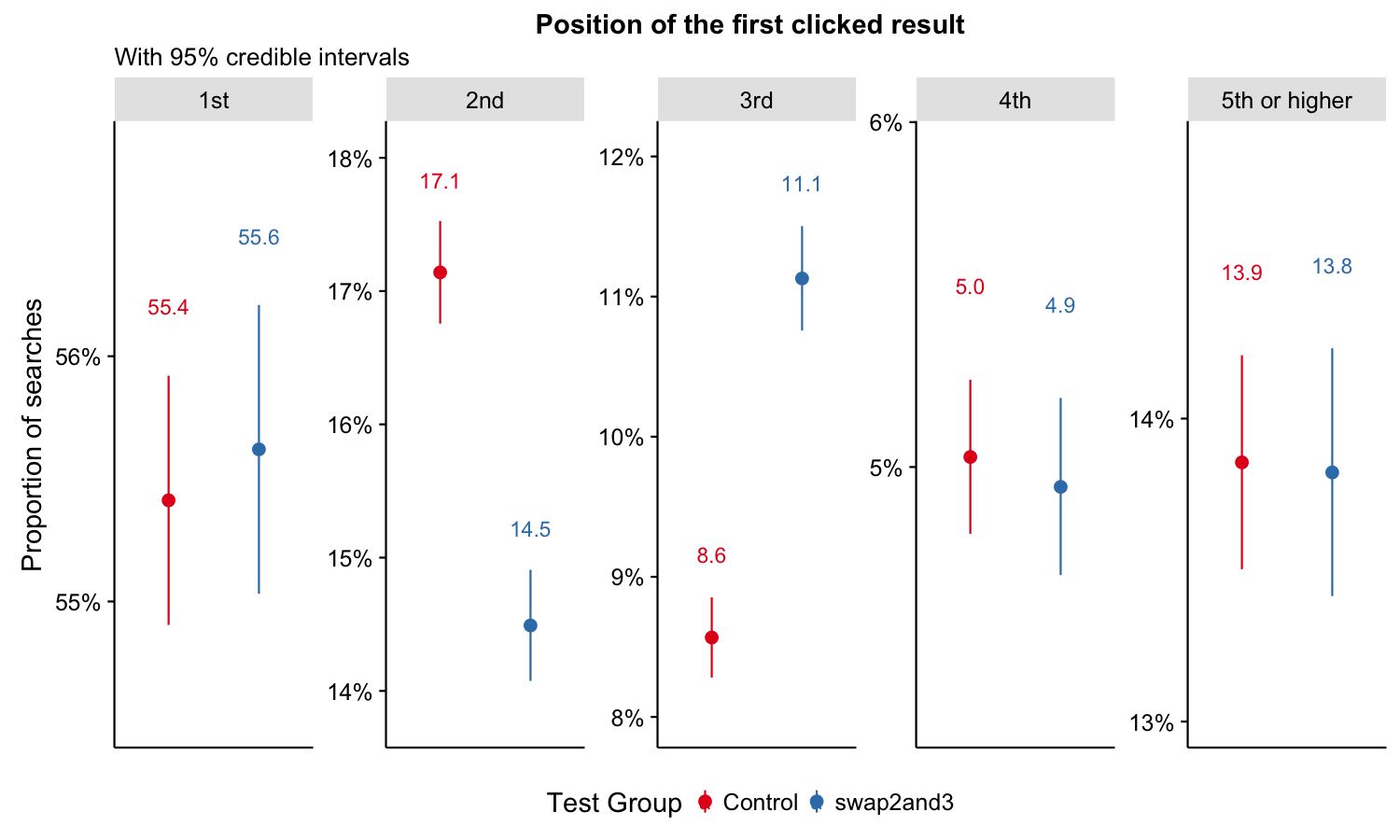
Figure 3: Proportion of searches that clicked a result first by position and group.
Dwell Time per Visited Page
When we compared the overall survival curves between the two groups, we found that the test group users were significantly more likely to stay longer on visited pages.
# Compare overall dwell time
temp <- clickedResults
temp$SurvObj <- with(temp, survival::Surv(dwell_time, status == 2))
fit_all <- survival::survfit(SurvObj ~ test_group, data = temp)
survminer::ggsurvplot(fit_all, conf.int = TRUE, xlab="T (Dwell Time in seconds)", ylab="Proportion of visits longer than T (P%)",
                      surv.scale = "percent", palette="Set1", legend="bottom", legend.title = "Test Group", legend.labs=c("Control","swap2and3"))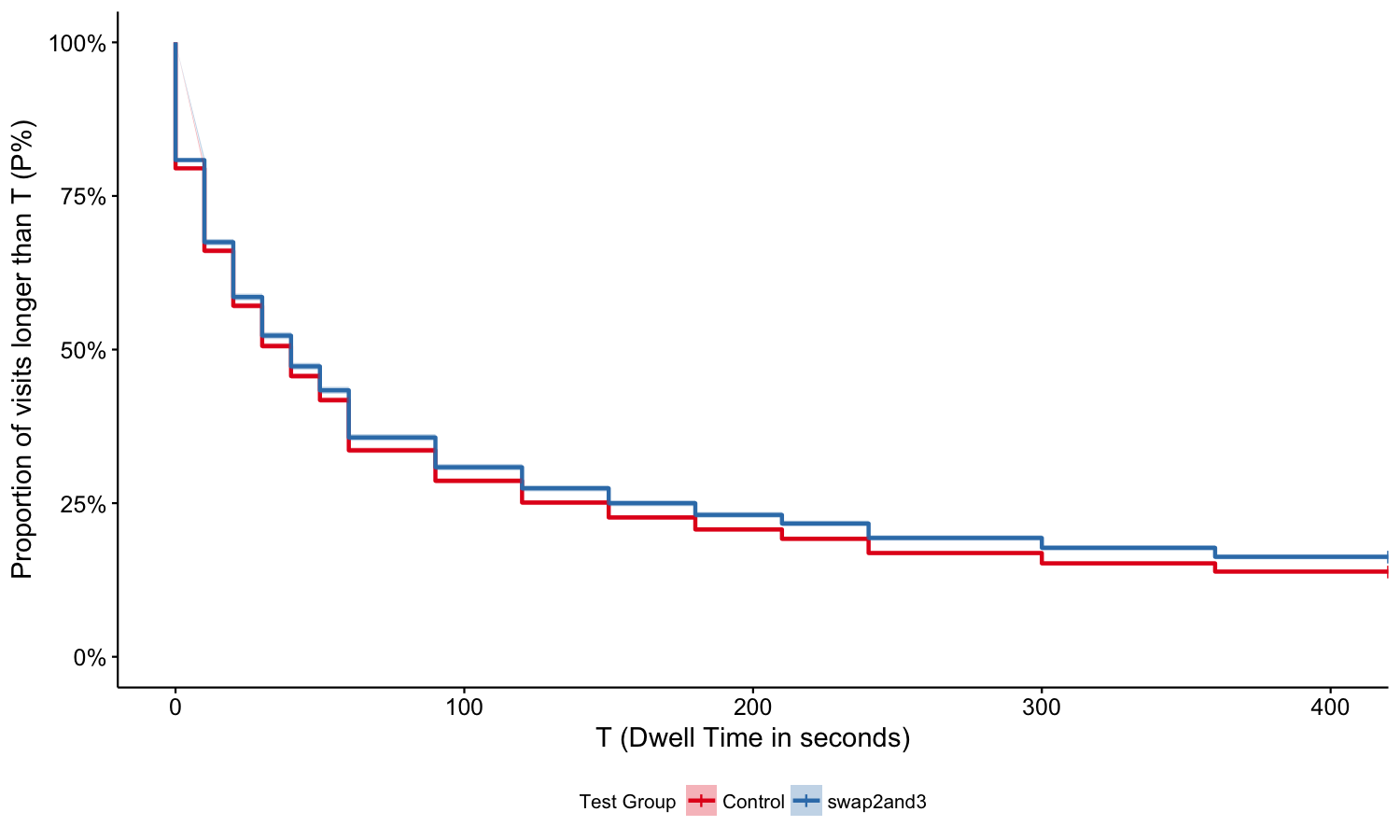
Figure 4: Survival curves with 95% confidence interval on visited pages after users click through, broken up by group. This shows the length of time that must pass before we lose 1-P% of the population. For example, it appears we have 80% of control group users stayed on visited pages by 10s.
rm(temp)When we compared the survival curves for users who clicked on the second or third result, we found that users in the test group who clicked on the 3rd result have a longer dwell time than others, but the difference is not significant.
temp <- clickedResults %>% filter(position %in% c(2,3)) %>%
  mutate(Test_Group = paste0(test_group, "(position ", position, ")"))
temp$SurvObj <- with(temp, survival::Surv(dwell_time, status == 2))
fit_2and3 <- survival::survfit(SurvObj ~ Test_Group, data = temp)
survminer::ggsurvplot(fit_2and3, conf.int = TRUE, xlab="T (Dwell Time in seconds)", ylab="Proportion of visits longer than T (P%)",
                      surv.scale = "percent", palette="Set1", legend="bottom", legend.title = "Test Group",
                      legend.labs=c("Control (position 2)","Control (position 3)","swap2and3 (position 2)","swap2and3 (position 3)"))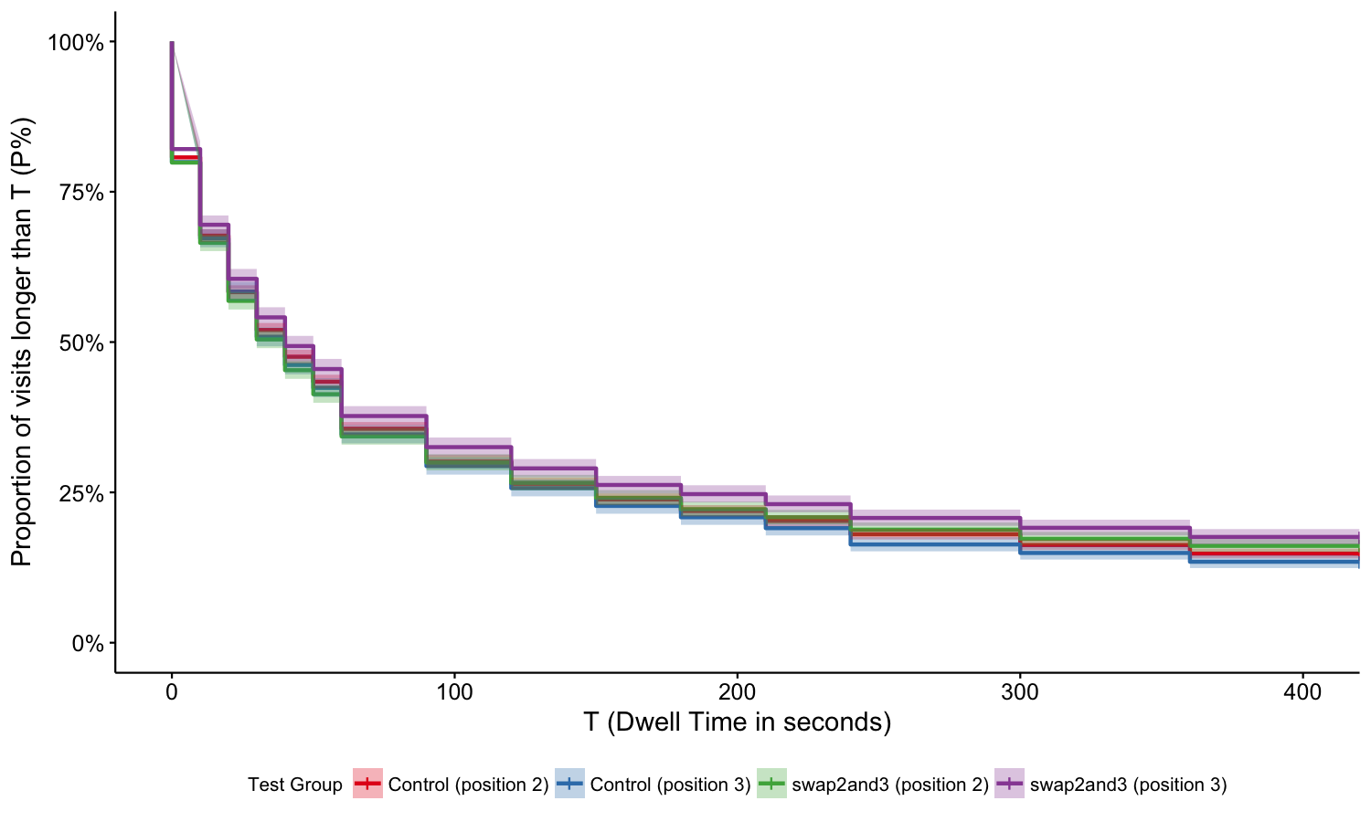
Figure 5: Survival curves with 95% confidence interval on visited pages after users click through, broken up by position and group.
rm(temp)Scroll
We found that users in the test group were significantly more likely to scroll on the visited page.
# Compare overall scroll proportion
scroll_overall <- clickedResults %>%
  group_by(test_group) %>%
  summarize(scrolls=sum(scroll), visits=n(), proportion = sum(scroll)/n()) %>%
  ungroup
scroll_overall <- cbind(
  scroll_overall,
  as.data.frame(
    binom:::binom.bayes(
      scroll_overall$scrolls,
      n = scroll_overall$visits)[, c("mean", "lower", "upper")]
  )
)
scroll_overall %>%
  ggplot(aes(x = 1, y = mean, color = test_group)) +
  geom_pointrange(aes(ymin = lower, ymax = upper), position = position_dodge(width = 1)) +
  scale_color_brewer("Test Group", palette = "Set1", guide = guide_legend(ncol = 2)) +
  scale_y_continuous(labels = scales::percent_format(), expand = c(0.01, 0.01)) +
  labs(x = NULL, y = "Proportion of visits",
       title = "Proportion of visits with scroll by test group") +
  geom_text(aes(label = sprintf("%.1f%%", 100 * proportion), y = upper + 0.0025, vjust = "bottom"),
            position = position_dodge(width = 1)) +
  theme(legend.position = "bottom")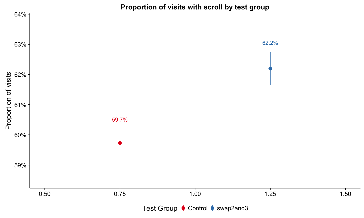
Figure 6: Proportion of visits with scroll by group.
Users in the test group who clicked on the 3rd result were significantly more likely to scroll on the visited pages than those who clicked on the 3rd result in the control group, but the differences were not significant in the 2nd result comparison and in the within-group comparisons.
# Compare position 2 and 3
scroll_2and3 <- clickedResults %>%
  filter(position %in% c(2,3)) %>%
  mutate(`Test Group` = paste(test_group, paste0("position",position), sep="_")) %>%
  group_by(`Test Group`) %>%
  summarize(scrolls=sum(scroll), visits=n(), proportion = sum(scroll)/n()) %>%
  ungroup
scroll_2and3 <- cbind(
  scroll_2and3,
  as.data.frame(
    binom:::binom.bayes(
      scroll_2and3$scrolls,
      n = scroll_2and3$visits)[, c("mean", "lower", "upper")]
  )
)
scroll_2and3 %>%
  ggplot(aes(x = 1, y = mean, color = `Test Group`)) +
  geom_pointrange(aes(ymin = lower, ymax = upper), position = position_dodge(width = 1)) +
  scale_color_brewer("Test Group", palette = "Set1", guide = guide_legend(ncol = 2)) +
  scale_y_continuous(labels = scales::percent_format(), expand = c(0.01, 0.01)) +
  labs(x = NULL, y = "Proportion of visits",
       title = "Proportion of visits with scroll by test group") +
  geom_text(aes(label = sprintf("%.1f%%", 100 * proportion), y = upper + 0.0025, vjust = "bottom"),
            position = position_dodge(width = 1)) +
  theme(legend.position = "bottom")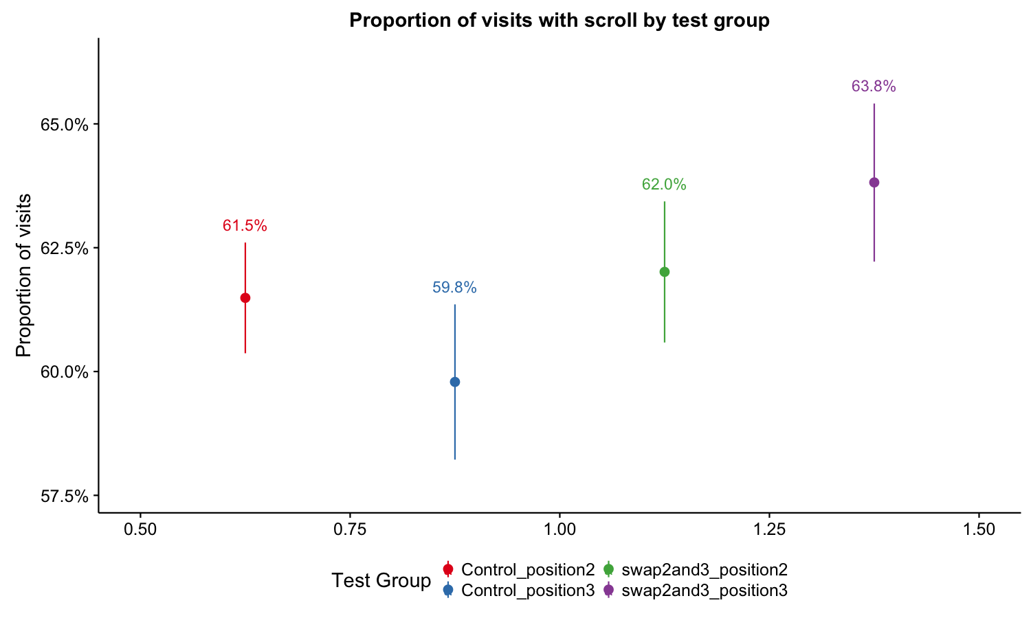
Figure 7: Proportion of visits with scroll by position and group.
Discussion
Overall, we found that user engagement decreased by swapping the second and the third search results. Position 2 had a higher clickthrough rate than position 3 in both groups. However, when comparing the same position between groups the clickthrough rate of third results in the test group was higher and the clickthrough rate of second results in the test group was lower. We also found that test group users were less likely to click on the 2nd result first than the control group, while they are more likely to click on the 3rd result first. Based on these analysis results, we believe that it is not an either/or situation with position (order displayed) and “quality” (as determined by Cirrus). We suspect that both position and quality matter in user behavior, but with different weights. Further experiments are needed to figure out the quantitative relationship between user behavior and these two factors.
It seems a little bit counter intuitive that the group with a lower engagement rate tended to stay longer and was more likely to scroll on the visited page, but we saw a similar case in another test before. This may be a case of the self-selection bias that users who click through in a probably less relevant group – the test group – may be different from users who click through in the control group in motivation, experience or other factors. Further research is needed.
Additionally, instead of making explicit control buckets, we simply treated those users who didn’t get assigned to the test group as control group users. We suspect that this behavior resulted in us putting all users whose browsers had a cached version of event logging JavaScript into the control group automatically, so some metrics may be biased.
References
Allaire, JJ, Joe Cheng, Yihui Xie, Jonathan McPherson, Winston Chang, Jeff Allen, Hadley Wickham, Aron Atkins, Rob Hyndman, and Ruben Arslan. 2016. Rmarkdown: Dynamic Documents for R. http://rmarkdown.rstudio.com.
Bache, Stefan Milton, and Hadley Wickham. 2014. Magrittr: A Forward-Pipe Operator for R. https://CRAN.R-project.org/package=magrittr.
Dorai-Raj, Sundar. 2014. Binom: Binomial Confidence Intervals for Several Parameterizations. https://CRAN.R-project.org/package=binom.
Keyes, Oliver, and Mikhail Popov. 2017. Wmf: R Code for Wikimedia Foundation Internal Usage. https://phabricator.wikimedia.org/diffusion/1821/.
Therneau, Terry M. 2015. A Package for Survival Analysis in S. https://CRAN.R-project.org/package=survival.
Wickham, Hadley. 2009. Ggplot2: Elegant Graphics for Data Analysis. Springer-Verlag New York. http://ggplot2.org.
———. 2017. Tidyr: Easily Tidy Data with ’Spread()’ and ’Gather()’ Functions. https://CRAN.R-project.org/package=tidyr.
Wickham, Hadley, and Romain Francois. 2016. Dplyr: A Grammar of Data Manipulation. https://CRAN.R-project.org/package=dplyr.